1
Young’s
Equation vs. Sessile Drop Accelerometry: A
Comparison Using the Interfacial Energies of Seven
Polymer-water Systems
Alfredo Calvimontes 1*
1 Predevelopment, Division Dish Care, BSH Hausgeräte GmbH (a subsidiary of Robert Bosch GmbH),
Robert-Bosch-Straße 16, 89407 Dillingen an der Donau, Germany
* Correspondence: [email protected]; Tel.: +49-9071-52-2410
Abstract: In this study, the values of the interfacial energies of seven different polymer-water systems obtained by Sessile Drop Accelerometry (SDACC) are compared with the values obtained by the Young’s-equation-based Owens-Wendt method. The SDACC laboratory instrument –a combination of a drop shape analyzer with high-speed camera and a microgravity tower- and the evaluation algorithms, are designed to measure the interfacial energies as a function of the geometrical changes of a sessile droplet shape due to the effect of “switching off” gravity during the experiment. The method bases on Thermodynamics of Interfaces and differs from the conventional aproach of the two hundred-years-old Young’s equation in that it assumes a thermodynamic equilibrium between interfaces, rather than a balance of forces on a point of the solid-liquid-gas contour line. A comparison of the mathematical model that supports the SDACC method with the widely accepted Young`s equation is discussed in detail in this study.
Keywords: surface energy, interfacial energy, surface tension, wetting model, wetting thermodynamics, sessile drop shape, microgravity
1. Background
Young [1] proposed two hundred years ago that the contact angle of the three-phase contact line results from the balance of three tensions. This idea can be expressed by the following equation:
Y L SL
S
cos
(1)where S, SL, and L represent the interfacial tensions per unit length of the solid-vapor, solid-liquid, and liquid-vapor contact line respectively, i.e. the surface tensions, and Y is the contact angle.
In principle, there are three important conditions for applying Young’s equation [2]: the surface has to be chemically homogeneous, completely flat and smooth, and the solid-liquid-vapor system must be free of the effects of gravity. Under these conditions, the Equation 1 represents the mechanical balance of three surface tensions along the contour line of the three phases. This balance has also been derived using the principle of minimizing the total free energy of the system [3-5]. Most recent thermodynamic derivation relies on interpreting S, SL, and L as scalar thermodynamic surface energies instead of tension vectors [4].
According to Makkonen [6], a very important reason for adopting the surface energy interpretation is that, while SL and L can be interpreted either way, the surface tension on a dry solid,S, is a contentious concept [3, 7-11]. Bikerman [8] and Ivanov et al. [9] have argued that Young’s equation is not a balance of forces. At the same time, the surface energy interpretation has led to many misunderstandings of the wetting phenomenon on patterned surfaces [12, 13]. The validity of Young’s equation was questioned [6]
According to Leger and Joanny, [19] the effect of body forces such as gravity on the contact line is small for small drop volumes. Gravity would affect the shapes of wetting liquid drops in their central region where they are flattened, but in a small region, close to the contact line, one would expect that the liquid-vapor and liquid-solid interfaces to make an angle given by the Young’s equation. These observations were supported by the theoretical calculations of Fujii and Nakae [20]. According to Leger, Joanny, Fujji and Nakae, only forces that become increasingly large at the contact line such as the viscous force on an advancing liquid can affect Young’s model. However, recent experimental evidence using microgravity by parabolic arc flights [21] and microgravity drop towers [22-23] have demonstrated that the effect of gravity on the contact angle is relevant even at very small drop volumes such as 5 µL. According to Allen [24], who studied the wetting of very small drops with small contact angles, a drop is small enough to neglect gravitational influences only if its volume is less than 1 µL.
Of the four parameters of Young’s equation, only L and Y can be readily measured; hence, this equation can only provide the difference between the solid-vapor surface tension S and the solid-liquid interfacial tension SL. For this reason, an additional equation providing a relation among the surface tensions in Young’s equation is required, i.e.,
)
,
(
S LSL
f
(2)Such an equation is referred to as an equation of state for interfacial tensions [25]. Combining Equation 1 with Equation 2, yield:
)
,
(
cos
Y S S LL
f
(3)This equation was the start point for several attempts to obtain mathematical expressions or numerical procedures able to provide the values of S and SL when only the values of L and Y are known. The most relevant solutions [26] were given by Fox and Zisman [27], Owens and Wendt [28], Janczuk and Bialopiotrowicz [29], Wu [30], van Oss, Chaudhury and Good [31], Li and Neumann [25], Kwok et al. [32], Shimizu and Demarquette [33] and Chibowski et al. [34]. Except for the Li-Neumann method, all the mentioned solutions use a pair or more liquids to calculate the surface energy of the solid and the interface solid-liquid. Experimental results of Hejda et al. [24] show that the solution of the mathematical approaches strongly depends on the liquids used. According to these authors, the approach proposed by Li and Neumann is also impractical because its strong dependence on the liquids used for the calculations.
More recently [35-37], a lab-scale microgravity tower was used to calculate the surface energies by means of sessile drops. This new method, the Sessile Drop Accelerometry (SDACC), revisit the phenomenon of wetting paying more attention to its surface nature as much as the derived approaches of Young’s equation have been put in the balance on the contact line of the three phases.
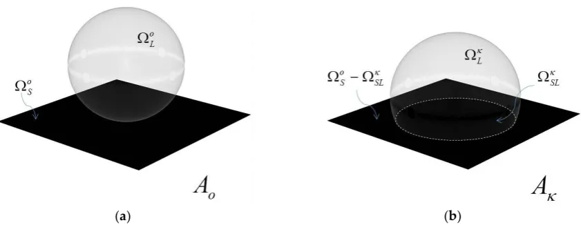
SDACC model considers a system where, in the initial condition that we will call the configuration o, the lower end of a liquid droplet is at an infinitesimal distance from a smooth solid flat surface of area oS
in a gas medium (Figure 1a). No force field is affecting the system (the acceleration of the system is zero, i.e. a*=0). Due to the absence of gravity, the shape of the droplet is a perfect sphere of area oL=4ro2,
where ro is the radius of the sphere. Under these conditions, and only due to the work developed by the
3
(a)(b)
Figure 1. In the absence of gravity, the droplet of the state Ao (a) spontaneously spreads on the surface and reaches the state A (b).
A quantity of importance in this analysis, as demonstrated above, is the change –the difference- of Helmholtz energy between each two contiguous j-configurations of the system during the spontaneous wetting process [38]. The term “configuration” refers to a state in which the droplet is at rest in a position of stable or metastable equilibrium. All the transient states among them are also thermodynamic configurations. Associated with each configuration are the characteristic interfacial areasjSL,jL and a characteristic Helmholtz energy, Aj.
For a given configuration for a one-component liquid, solid and gas, at constant temperature and volume [35, 37]:
i j
j
A
(
)
(
)
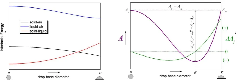
(4)where is the scalar thermodynamic surface energy that characterizes the thermodynamic property of an interface. Let’s take as an example a system in which L > SL > S. During the spontaneous wetting of
the droplet of Figure 1, the Helmholtz energy of the system decreases because part of the liquid-gas interface creates a new solid-liquid interface (Figure 2, left). The energy of the solid-gas interface contributes additionally to the creation of the solid-liquid interface. The wetting process ends when the system reaches the equilibrium in the configuration .
The wetting process could end precisely at the configuration d`, where the Helmholtz energy of two contiguous j-configurations presents no more change (Aj = 0). However, the internal energy stored inside the drop during the wetting between o and d’ can make the work necessary to continue wetting from d’
up to the equilibrium configuration , i.e., E = A – Ad’. At this point, the configuration , the Helmholtz energy of the system recovers the value of the initial configuration o. In other words, comparing the configurations o and , no work has been done on the system, nor has it done any work on its surroundings. The net change of Helmholtz energy during the wetting process is zero.
0
A
oA
A
o (5)Figure 2. Schematic representation of the energetic changes of a system while a drop spontaneously wets a solid surface without the effect of gravity.
Continuing with the ideal model of spontaneous wetting, from Equation 4:
0
oS S o L L SL o S S SL SL L L o
A
(6)That results in:
0
o SL S SLL L
L (7)
A parameter can be now defined as:
SL L o L
(8)is a dimensionless parameter that characterizes a liquid drop at equilibrium resting on a flat surface without the effect of gravity. Under the condition of weightlessness, this parameter is, in principle, independent of the size of the drop and not equivalent to the cosine of the contact angle of Young’s model:
L S
SL
(9)In the Young’s model, cosY represents the bi-dimensional fraction of the liquid surface tension acting horizontally on the triple contact point solid-liquid-gas. By contrast, for SDACC, represents the ratio of the liquid-gas interface area-decrease and the solid-liquid interface area created by wetting (Eq. 8). In other words, for a defined solid surface, represents the balance between the surface tension of the liquid and the interfacial solid-liquid energy. While cosY applies only to the boundary line of the bi-dimensional drop profile, applies to all the interfaces of the three-dimensional system.
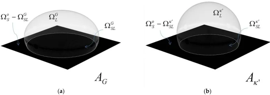
Let’s consider now another wetting process. As initial condition –configuration G-, a drop is resting in equilibrium on a solid and flat surface under the effects of the terrestrial gravitational field (a1=-gE,
gE=9,81m/s2), see Figure 3a. Suppose that the system is inside a closed capsule that is submitted to the free fall under controlled conditions.
If a2 is the acceleration of the uniformly accelerated motion of the capsule downwards, in the case of the free fall, its value is obviously –gE. This will switch off the effects of the gravitational field inside the capsule that contains the surface and the drop. The resulting acceleration of this system will be given by:
1 2 *
a
a
5
(a) (b)
Figure 3. By the free fall, the energy that the terrestrial gravitational field is producing on the droplet (a) is released, letting the droplet reach a new equilibrium only governed by the interfacial energies (b), which shape is a spherical dome.
So, in the case of free fall, a* = 0, that corresponds to an inertial system inside the capsule. To reach this condition, the energy with which the terrestrial gravitational field is flattening the drop must be released, letting the drop reach a new equilibrium state (Figure 3b) only governed by the interfacial energies –the configuration '-. Macroscopically, it will result in the receding of the drop by the decrease of the interfacial area and its “deformation” to a perfect sphere due to the increase of its height. The acceleration that modifies the drop shape during the very short time of the mentioned energy release process is given by af:
2
a
a
f
(11)During the energy release process, the receding of the drop will result in contact angle hysteresis. The multiplicity of apparent contact angles, which is an essential feature of contact angle hysteresis, is associated with the multiplicity of equilibrium states that a drop may assume on a rough or heterogeneous surface [39]. One apparent contact angle is associated with the stable equilibrium state (the global minimum in the free energy of the system). The others are linked to metastable equilibrium states (local minima in the free energy). The transition between metastable states, toward the stable equilibrium state, depends on the energy available to the drop for overcoming the energy barriers which inherently exist between the metastable states [39].
By definition, the phenomenon of hysteresis is observed when a parameter of the system, such as the volume of a drop placed on a solid, is varied back and forth, or when an external force is making the drop move in one direction (ie., by the tilting table experiment). In SDACC, the release of gravitational energy makes the contour of the drop recede on the surface and experience hysteresis. For this reason, this microgravity model is, in principle, oriented to characterize chemically homogeneous and smooth surfaces.
Going back to the case of the sessile drop in the free fall, the acceleration experienced by the drop for the short time of the energy release is af = +gE, i.e., a short duration force acting upwards. The mechanical work that the drop must make to modify its shape and release surface energy is given by WM.
G
M
A
A
A
W
' (12)From the standpoint of the drop, this work can also be divided into two components: the work WP necessary to move up its center of mass and the work WS necessary to radially move the contour line solid-liquid-gas during a short de-wetting process (Figure 4).
S P
M
W
W
W
(13)Figure 4. The free-fall makes the system release the energy with which the gravitational field was deforming the drop. The Helmholtz energy of the drop in the form of interfacial energies is released, resulting in a drop with a spherical dome shape, the configuration '.
The change in the potential energy of the droplet can be calculated by measuring the change in the position of all the liquid particles, by considering for a moment the liquid as a particle system. If a particle system is changing from the state 1 to the state 2, their potential energies under a force field that produces the acceleration af, can be described by:
ni
i f i
p
m
a
z
e
1 1 (14)
ni
i f i
p
m
a
z
e
2 2 (15)Where mi is the mass of each particle, zi its vertical position, and n the total number of particles. The
7
ni i i n i i i f
p
a
m
z
m
z
W
2 1 (16)The center of mass of a particle system is defined by:
m
z
m
z
n i i i c
(17)Then, the Equation 16 for the potential energy necessary to move all the liquid particles from the state G to ', can be written as:
c cG
f
c cG
f
p
m
a
z
z
V
a
z
z
W
'
'
(18)Where is the density of the liquid and V is the drop volume.
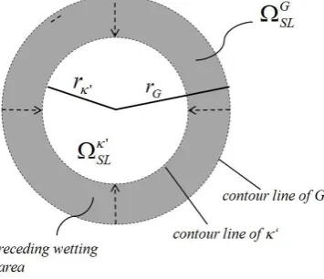
The second component of the work that the drop must make, the energy necessary to produce the receding wetting during its deformation from the state G to ', can be calculated by the integration of all the differentials of energy needed to move the contour line on the surface in the radial direction (Figure 5):
Figure 5. The drop profile observed from above: the release of the force field leads to dewetting. A receding work decreases the interfacial area fromGSL to'SL.
' '
G Gs
l
dr
dW
(19)Where is tension necessary for the drop to move the contour line on the surface, l is the length of the contour line and r the radius of the wetting area SL. These considerations result in:
'2
Gs
r
dr
W
(20)Which, in turn, results in:
G
SL SL G
s
r
r
W
2'
2
'
(21)At the equilibrium, the work made by the drop –the energy released- will result in energy changes on the system surfaces. Equations (12), (13), (18) and (21) result in:
G
SL o S SL o S S G SL SL SL G L L L G SL SL cG cf z z
a
V
' ' ' ' ' (22)
Making the corresponding arrangements:
f
c cG
G L L L G SL SL S
SL
V
a
z
'
z
' '
(23)In the case of a free fall, both terms at the left side of Eq. 22 must give negative values because the drop must release energy to deform its shape, i.e. it must do work. By the first term, the acceleration and the difference of center of mass are both positive, resulting in a negative term due to the minus sign ahead of it. The second term is also negative, because the minus sign, the negative value of the areas difference – receding wetting- and the value of , which is negative due to the following reason: during the dewetting of the drop contour, the tension is the force that the liquid must overcome to recede on the solid surface, i.e., to “create” solid surface. This surface tension is the opposite of the previously defined surface energy of the solid S:
S
(24)Under this consideration, the Equation 23 can be written as:
fall
free
g
a
z
z
Va
E f G SL SL G L L L cG c f SSL
2
',
,
' '
(25)Summarizing, in the case of the free fall, a2 = -gE (capsule is falling) and a1 = -gE (terrestrial acceleration acting on the droplet in rest). So, the net acceleration that deforms the droplet for a very short time during the free fall is af = +gE, i.e. a short duration deformation force from bottom to up. However, once the drop reaches the equilibrium inside the capsule, it will be found within a system with zero acceleration, ie. a* = 0 (weightless). In consequence, at the end of the experiment (configuration ’), the drop will be resting in stable equilibrium inside an inertial system.
The configuration , as mentioned before, is reached ideally after the end of a very fast wetting process that started spontaneously with the configuration o without the effect of the gravity. In the microgravity method, however, the configuration is quantified in a special way: the capsule with a drop in the configuration G, i.e., resting under the effects of the terrestrial gravity (a1=-gE, gE=9,81m/s2) is moved downward with a2=-gE, (free fall). This results, as seen above, in a sudden upward acceleration af =+gE that deforms the drop for some moment (milliseconds in practice) until it reaches the weightlessness state (a*=0) inside the capsule (inertial system), the so-called configuration ’. The present model proposes that the configuration ’ resulting from this forced de-wetting process is the same as the configuration , or at least quite similar.
By analyzing the images provided by the high-speed camera using Axisymmetric Drop Shape Analysis (ADSA) or ellipse matching, it is possible to find the frames where the droplet is resting free of vibrations with a perfectly spherical shape (the ellipse matching is highly recommended). These images correspond to the configuration =’ of the SDACC model. The values of the interfacial areas oL,L,
and SL can be obtained by the drop volume, the matching method and the formulas presented in [35, 37], to obtain the value of the parameter , using the Eq. 8.
9
technology with SDACC could make possible its application for non-axisymmetric drops on anisotropic surfaces.
The values of the interfacial areas GL, and GSL can be obtained from the first frames some milliseconds before starting the free fall. This instant corresponds to the drop resting in equilibrium under the effects of gravity, the configuration G. The drop centers of mass zCG and zC' can be calculated from the initial images and the images of configuration =’, by applying the equations presented in [35, 37]. The exact value of the acceleration af, can be obtained from the accelerometer of the instrument (see the Experimental Section).
The values of S and SL can be obtained by solving the system given by the equations 9 and 25. For
the application of the microgravity method, it is only necessary to know the value of the surface tension of the liquid, its density, and the drop volume.
The precision of SDACC is highly dependent on the precision of the interfacial areas measurement. During the energy release of the drop, it could move some micrometers on the camera view-axis. As a consequence, the scale of the frames could change a little bit during the process. For this reason, the drop shape matching algorithms must be carefully scaled to evaluate the drop shapes of the configurations =’
and G with constant drop volume.
The artificial accelerations produced inside the capsule result in drop deformations given by af. Two cases of spheroidal caps (sphere and oblate) must be differentiated to calculate the values of the solid-liquid SL and the liquid-airL interfacial areas: a*=0 and a*<0 [35, 37].
2. Experimental Section
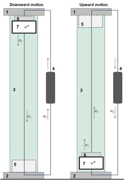
The instrument [35] consists of a vertical tower three meters tall with all the necessary elements to control the accelerated movement of a capsule containing the solid-liquid-gas system during a time span from 600 to 750 milliseconds. The tower (Figure 7) was originally constructed to allow the motion of the capsule under different acceleration values upwards and downwards. However, the present study is focused on the free-fall mode, i.e. the instrument as a microgravity tower.
The components of the instrument are: the upper ignition device (1), the lower ignition device (2), the displacement tower (3), the acceleration device (4), the braking or damping mechanism (5) the liquid dosing device (6) and the capsule with the sample (7). Further, the instrument is connected to a computer with the software necessary to control the devices and evaluate the data.
The upper ignition device (1), as well as the lower ignition device (2), are electromagnetic mechanisms designed to release the anchored capsule so it can move freely by the action of the acceleration device. They are designed to minimize the vibrations during the ignition. The displacement tower (3) is designed to guide the capsule in the vertical direction without vibration and minimizing the effects of friction. The acceleration device (4) actuates the capsule in values of constant acceleration using the linear increase of the speed starting from the rest (zero velocity). This device is capable of moving the capsule both upwards and downwards. In the case of the downward drive with the acceleration of –gE (Earth gravitational field), it is possible to let the capsule simply fall free with the help of the guide elements of the shift tower. The acceleration device may be a servo motor capable of producing constant accelerations upwards or downwards of any value or a mechanical device which, based on a combination of pulleys, moves the capsule in discrete acceleration values.
Figure 7. The measure capsule (7) can be moved upwards or downwards.
The liquid dosing device (6) must be able to dose small droplets from 5µL to 100µL on the sample surface inside the capsule. It can consist of an arrangement of a micro-pump and dosing cannula or a mechanic or electronic micropipette. In the first case, it could be attached and moved together with the microcapsule. In the case of a micropipette, it could be triggered independently of the tower structure.
11
The measuring capsule consists of a high-speed camera (100 – 1000 frames per second, fps), a sample stage (XYZ), a diffuse light source, an accelerometer, a vibrometer and a refrigeration unit (ventilator) (Figure 8). This device can obtain images or video of the drop during its motion with good resolution at higher fps values. The diffuse light must provide a good illumination and allows a good contrast to obtain sharp drop contours. The stage will be used to put the sample in the optimal position for the experiment. The accelerometer and the vibrometer measure the values of the acceleration (Z-Axis) inside the capsule and the values of the accelerations in X- and Y-axis to evaluate the vibration during the experiment, respectively. The ventilator is used to cool the high-speed camera between the measurements.
The first published results of SDACC [35] were realized using polypropylene (PP) and polytetrafluoroethylene (PTFE) surfaces. In [37], more tests realized using seven smooth polymer surfaces -including new PP and PTFE-, were reported. This data will be analyzed in more detail in the present study.
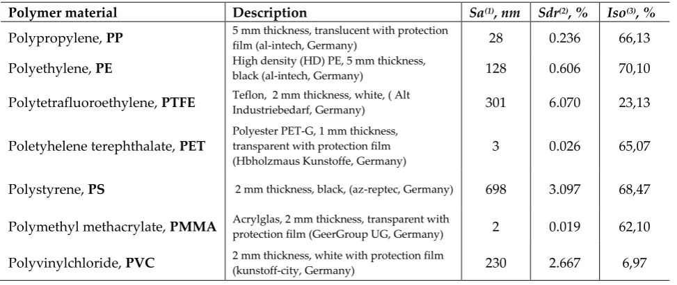
The topographic parameters of the seven polymer surfaces are listed in Table 1.
Table 1. Polymer surfaces and roughness
Polymer material Description Sa(1), nm Sdr(2), % Iso(3), %
Polypropylene, PP 5 mm thickness, translucent with protection film (al-intech, Germany) 28 0.236 66,13
Polyethylene, PE High density (HD) PE, 5 mm thickness, black (al-intech, Germany) 128 0.606 70,10
Polytetrafluoroethylene, PTFE Teflon, 2 mm thickness, white, ( Alt Industriebedarf, Germany) 301 6.070 23,13
Poletyhelene terephthalate, PET
Polyester PET-G, 1 mm thickness, transparent with protection film (Hbholzmaus Kunstoffe, Germany)
3 0.026 65,07
Polystyrene, PS 2 mm thickness, black, (az-reptec, Germany) 698 3.097 68,47
Polymethyl methacrylate, PMMA Acrylglas, 2 mm thickness, transparent with
protection film (GeerGroup UG, Germany) 2 0.019 62,10
Polyvinylchloride, PVC 2 mm thickness, white with protection film (kunstoff-city, Germany) 230 2.667 6,97
1 Surface arithmetic mean roughness; 2Developed surface area ratio; 3Texture Isotropy
The topographic characterization was carried out using high-resolution ScanDisk Confocal Microscopy (SDCM). The SDCM device was a µsurf explorer (Nanofocus AG, Germany). An objective with the magnification 100X was used, which provides a measure length of 160 µm and lateral and vertical resolutions of 0.3 µm and 2 nm respectively. Three measurements were carried out on different positions of the samples. The topographic parameters arithmetic mean roughness Sa and developed surface area ratio Sdr (Table 1) show that the roughness of the materials is small enough to consider the surfaces smooth for the experiments. The texture isotropy, calculated using the MountainsMap® Premium Software (Digital Surf sarl, France) show that the PP, PE, PET, PS and PMMA surfaces are isotropic enough to consider that the drop will form axisymmetric shapes. The morphology of these surfaces was only slightly affected by negligible scratches due to manipulation. In case of PTFE and PVC, however, the anisotropy is structural. However, the nanometric- scale roughness of these surfaces, 301 and 230 nanometers respectively, should not significantly affect the axisymmetry of the 15 µL water droplets (approx. 4-5 mm of base diameter) that will be deposited on them.
The materials were cut into 5 x 5 cm2 samples and submitted to the tests with the microgravity lab
3. Results
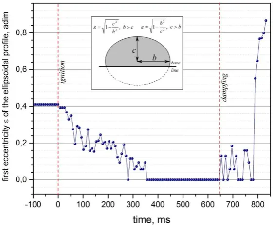
The calibration of the apparatus was realized according to [35]. To quantify the stabilization time of the droplets during the experiment, the first eccentricity was used [35]. A perfect sphere with zero eccentricity in the microgravity region confirms that the effects of vibration were released. According to Figure 9, the eccentricity for doubled distilled water droplets of 20 µL on the PP surface shows that the vibration is completely released after 350 milliseconds of the ignition.
Figure 9. Vibration release of water drops on a PP surface regarding drop shape eccentricity. 76 frames were analyzed from the 480 available (750 fps video recording) [35].
The calculation of the interfacial areas is possible using the equations presented [35]. The values obtained for the parameter ’ on all the seven surfaces are listed in Table 2. Ten measurements corresponding to ten different drops were made for 15 µL bi-distilled water droplets on each surface at 22±1 °C of temperature and 60±2 % of relative humidity. According to [35], the optimal volume for the experiment using water is between 10 and 20 µL because in this interval both, the surface tension and the gravitation, are governing the wetting and the drop shape. According to [22], there are two forces that principally produce the droplet shape: the surface tension of the liquid, which tends to minimize the area of the surface (producing the spherical shape) and the gravitational force which tends to flatten the droplet.
Before initiating the free fall, the interfacial areas at the G-configuration, i.e. the sessile droplet under the effects of the gravity, were measured using the droplet images. The droplet mass centers in the G and
' configurations were also measured for each experiment. The interfacial energies were calculated by solving the system given by the equations 9 and 25 for each experiment, i.e., for each pair of images corresponding to the G and ’ configurations. The results are presented in Table 2.
During the free fall, the water droplet experienced receding wetting during approximately 450 milliseconds in case of the PP surface [35]. During this period, the system went through multiple transient and metastable states. The oscillations due to the energy barriers of the surface combined by the mechanical micro vibrations due to the electromagnetic release of the capsule lead the droplet to the equilibrium (’) through multiple metastable states.
13
Polymer
'
S , mJ/m2
SL, mJ/m2
Polypropylene, PP 0.5287 ± 0.0058 30.8708 ± 0.4070 69.3591 ± 0.2354 Polyethelyne, PE 0.4030 ± 0.0127 34.0385 ± 0.5512 63.3805 ± 0.7212 Polytetrafluoroethylene, PTFE 0.6199 ± 0.0037 20.1871 ± 0.5006 65.3167 ± 0.5071 Poletyhelene terephthalate, PET 0.3564 ± 0.0123 41.3845 ± 0.3405 67.3328 ± 0.9448 Polystyrene, PS 0.3376 ± 0.0372 43.4610 ± 0.7066 68.0411 ± 2.5544 Polymethyl methacrylate,
PMMA 0.1528 ± 0.0192 49.2423 ± 0.6394 60.3631 ± 0.9917
Polyvinylchloride, PVC 0.3764 ± 0.0073 34.5522 ± 0.4563 61.9534 ± 0.4893
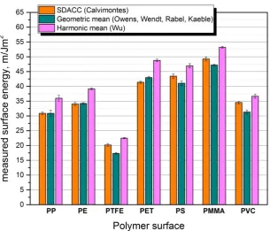
To compare the microgravity method with the Owens-Wendt [28] and Wu [30] methods, measurements with a Mobile Surface Analyzer –MSA (Krüss GmbH, Germany) were realized using doubled distilled water and diiodomethane (Sigma-Aldrich). For each of the seven surfaces, ten drops of 1µL were used. The results are presented in Figure 10.
Figure 10. Comparison between the calculated values of S for the seven polymer surfaces obtained by the methods Owens et al., Wu, and SDACC.
4. Discussion
According to the results, the SDACC correlates well with the results obtained by the method of Owens et al. [28] for Polypropylene (PP), Polyethylene (PE) and Polyethylene terephthalate (PET). The values obtained for the surfaces of Polytetrafluoroethylene (PTFE), Polystyrene (PS), Polymethyl methacrylate (PMMA) and Polyvinylchloride (PVC) are intermediate between the values obtained by the methods of Owens et al. and Wu. In all the cases, the values obtained by Wu tend to be considerable higher.
As mentioned above, recent experimental evidence using microgravity by parabolic arc flights [21]
relevant even at very small drop volumes such as 5 µL. According to Allen [24], who studied the wetting of very small drops with small contact angles, a drop is small enough to neglect gravitational influences only if its volume is less than 1 µL. In [37], the eccentricity of small droplets of only 1µL was used to demonstrate quantitatively that the effects of the gravity are still significant on very small droplets.
The deforming effect of the gravity on the droplet is not the only problem for determining the interfacial energies using the contact angle methods like Owens et al. and Wu. The use of small droplets leads additionally to the increase of the effects of the roughness on the contour line. Even smooth surfaces have micro- and nanometric inhomogeneities that could affect the solid-liquid-gas contour line of the droplet. And this is very relevant when the method used is based only on the geometry of the boundary solid-liquid-gas.
As mentioned above, in Young’s model cosY represents the bi-dimensional fraction of the liquid surface tension acting horizontally on the triple contact point solid-liquid-gas. By contrast, in SDACC, represents the ratio of the liquid-gas interface decrease and the solid-gas interface created by wetting (Eq. 8). While cosY applies only to the boundary line of the bi-dimensional droplet profile, applies to all the interfaces of the three-dimensional system.
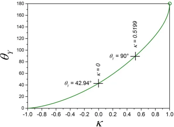
A relationship between and Y can be built by means of a mathematical simulation considering a spherical drop of any liquid that virtually wets and spreads from = 180° to = 0° on any smooth surface in absence of gravity. By the definition of Young’s equation, Y = , because the Young’s model considers no effect of gravity. According to Figure 11, the relationship between Y and is near to an exponential with a -domain [-1; 1[. If Y 180°, then 1. But if Y =180°, is not defined because it results in a division by zero, according to Eq. 8, where, in this case, the interfacial area solid-liquid does not exist anymore.
Figure 11. The relationship between Young’s contact angle (considering weightless, Y= ) and the
parameter .
15
liquid-air interfacial area of the original spherical drop before wetting. As mentioned before, by the Young’s equation (Eq. 1), if the surface energy (in mJ/m2) of the solid equals the tension (in mN/m) of the
solid-liquid contour, then the contact angle is 90 degrees (cosY = 0), while by SDACC, the surface energy of the solid equals the energy of the solid liquid interface only if = 0. The contact angle, in this case, is
= 42.94°. This value is the threshold hydrophobicity-hidrophilicity of the thermodynamic model for SDACC.
Young’s model considers an interfacial solid-liquid tension on the contour line. Let’s rename this parameter SL(Y) to differentiate from the interfacial energy SL defined for SDACC. By combining the Equations 1 and 9:
Y
L Y SL
SL
( )
cos
(26)According to Equation 26, there is a difference between the interfacial energies measured on the interfacial area solid-liquid (SL) and on the contour line (LS(Y)) solid-liquid-gas. This difference is controlled by the liquid surface tension and by + cosY. Figure 12 shows the behavior of this difference as a function of Young’s contact angle. According to this, the interfacial energy solid-liquid measured by Young’s model on the contour line is only valid for the solid-liquid interface in the case of complete wetting (Y = 0°).
By Young’s model, complete wetting means S(Y) = SL(Y) + L, because the contact angle is zero (cosY = 1). In this wetting case, SDACC predicts = -1, which leads to S = LS + L. According to this, at complete wetting both models match, ie. SL = SL(Y). At the opposite end, by Y = 180° (cosY = -1), the Young’s model predicts that S(Y) = SL(Y) -L, that means that SL(Y) =L, because, by definition, S(Y) is zero by non-wetting. By SDACC, non-wetting means that tends to one (see Figure 14). While in this case, S tends to zero, thenSL tends to L (see Eq. 25), practically in agree with Young`s wetting model.
As can be seen, SDACC and Young`s model agree at the limits of complete wetting and non wetting. However, both models predict quite different behaviors among these limits. These differences can be quantified by + cosY (see the red curve in Figure 12), that, multiplied by the surface tension of the liquid (see Eq. 52) results in the difference between the interfacial energy solid-liquid measured on the interface (SL), and on the contour line (SL(Y)).
Table 3. Results of the surface characterization using the Young’s-based Owens et al. method [28] under the effects of terrestrial gravitation(
L = 72.8 mJ/m2).Polymer
cos
Y
S(Y) , mJ/m2
SL(Y), mJ/m2
Polypropylene, PP -0.0507 ± 0.0207 30.886 ± 0.9987 34.5789 ± 2.0187 Polyethelyne, PE -0.0294 ± 0.0167 34.221 ± 0.2809 36.3591 ± 1.2635 Polytetrafluoroethylene, PTFE -0.2958 ± 0.0159 17.300 ± 0.2592 38.8343 ± 1.2477 Poletyhelene terephthalate, PET 0.2225 ± 0.0140 42.978 ± 0.3877 26.7801 ± 0.9510 Polystyrene, PS 0.2487 ± 0.0332 41.043 ± 0.7155 22.9402 ± 2.0187 Polymethyl methacrylate,
PMMA 0.3081 ± 0.0129 47.204 ± 0.2448 24.7717 ± 0.8288
Polyvinylchloride, PVC -0.0542 ± 0.0437 31.298 ± 0.7157 35.2409 ± 2.7093
The surface characterization of the polymers by the Owens et al. method [35] provided the results listed in the Table 3.
As seen in the Figure 10 and according to the data presented in the Table 2 and Table 3, the measured values of the surface energy of the solids are very near, in some cases practically the same, by using SDACC and Owens et al. methods. However, the values of the interfacial energy solid-liquid are quite different because SDACC measures the energy in the interface solid-liquid, while the Young’s-based Owens et al. method measures the interfacial energy exactly on a point of the contour line liquid-gas. In all the cases, the interfacial energies are larger while measured below the droplet, ie. on the solid-liquid interface. Table 4 presents the differences between the interfacial energies measured by both methods.
Table 4. Differences between the surface characterization parameters using SDACC and the Young’s-based Owens et al. method(
L = 72.8 mJ/m2).Polymer
deg*
Y deg**
S
S(Y) mJ/m2
SL
SL(Y) mJ/m2
Polypropylene, PP 90.99 92.91 -0.0152 34.7802
Polyethelyne, PE 77.76 91.69 -0.1825 27.0214
Polytetrafluoroethylene, PTFE 101.52 107.23 2.8871 26.4824
Poletyhelene terephthalate, PET 73.15 77.13 -1.5935 40.5527
Polystyrene, PS 71.54 75.51 2.4180 45.1009
Polymethyl methacrylate, PMMA 54.93 72.04 2.0383 35.5914
Polyvinylchloride, PVC 75.07 93.12 3.2542 26.7125
* 15µL water droplets, weightless ** 1µL water droplets, gravity
17
hydrophobic (S < SL). But, if ‘< 0, then ' < 42.94°, and S > SL, according to Equation 9. This condition -the hydrophilicity by SDACC- would increase wetting easily by applying a gravitational force and, in consequence, decrease considerably the contact angle (see the explanation of Figure 13).
(a) (b) (c)
Figure 13. The effect of gravity on the contact angle depends on the value of ', which defines the threshold ' = 42.94°. (a) and (b) represent the case ' > 0. The case (c) occurs if ' <0. Only in this case the gravity leads to a smaller contact angle than the microgravity.
Figure 14. Relevant parameters of SDACC for a 1 mm radius droplet that wets a smooth surface.
5. Conclusion
The experimental results of surface and solid-liquid interfacial energies corresponding to seven different smooth polymers were compared with the measurements using the Owens et al. method based on the Young’s equation. The results show that SDACC provides similar values of solid-gas surface energies to those obtained by Owens et al. with good reproducibility. However, in compare with the Young’s equation based method, the thermodynamic model that supports SDACC allows the accurate and direct measurement of the true interfacial solid-liquid energy and not only the value of the tension on a point of the solid-liquid-air contour line. This is the most important advantage of SDACC over Young’s equation based methods. Another very important advantage is to allow the accurate study of wetting phenomena without the effect of the terrestrial gravity.
In all the studied polymer-water systems, the interfacial energies were larger while measured below the droplet, ie. on the solid-liquid interface than on the solid-liquid-gas contour line.
For the application of the method, only one liquid with a known value of surface tension is needed. The values of the interfacial energies can be obtained by solving a linear system of two equations. No correlations or numerical methods are needed. The vibrations produced during the start of the wetting process are successfully controlled by the electromagnetic release of the drop tower. The experimental results are showing that the release of these vibrations occurs for a very short time and could help the receding wetting. The high-speed camera of the instrument allows obtaining images of the droplets for an additional time free of vibrations. The effect of the receding wetting during the experiment and its implication on the results was also discussed in this study.
In contrast to the universally accepted boundary wetting threshold of 90 degrees (Young’s model), the model of SDACC proposes that the thermodynamic interfacial wetting threshold between hydrophobic and hydrophilic characters occurs when the contact angle on the drop boundary is 42.94 degrees (SL = S).
The instrument and its evaluation method open new possibilities to develop surface characterization procedures by submitting the solid-liquid-system to artificial generated and uniform force fields.
Conflicts of Interest: The author declares no conflict of interest.
References
1. Young, T. An Essay on the Cohesion of Fluids. Phil. Trans. R. Soc. Lond. 1805, 95, 65-87
2. Sheng, Y. J.; Shaoyi, J.; Tsao, H. K. Effects of geometrical characteristics of surface roughness on droplet wetting.
The Journal of Chemical Physics 2007, 127, 23, 4704-7
3. Gibbs, J. W. The Scientific Papers of J. Willard Gibbs, Thermodynamics vol 1. Dover Publications, New York, 1961 4. Whyman, E.; Bomarschenko, G.; Stein, T. The rigorous derivation of Young, Cassie-Baxter and Wenzel equations
and the analysis of the contact angle hysteresis phenomenon. Chem. Phys. Lett. 2008, 450, 355-359
5. Roura, P.; Fort, J. Local thermodynamic derivation of Young’s equation. J. Colloid Interface Sci. 2004, 272, 420-429 6. Makkonen, L. Young’s equation revisited. J Physics.: Condens Matter 2016, 288, 135001
7. Orowan, E. Surface energy and surface tension in solids and liquids. Proc. R. Soc. A 1970, 316 473-91 8. Bikerman, J. Surface energy of solids.Top. Curr. Chem. 1978, 77 1-66
9. Ivanov, I. B.; Kralchevsky, P. A.; Nikolov, A. D. Film and Line Tension Effects on the Attachment of Particles to an Interface. J. Colloid Interface Sci. 1986, 112 97-107
10. Makkonen, L. Misinterpretation of the Shuttleworth equation. Scr. Mater. 2012, 66, 627-9
11. Makkonen, L. Misconceptions of the Relation between Surface Energy and Surface Tension on a Solid. Langmuir
2014, 30 (9), 2580-2581
12. Gao, L.; McCarthy, T. J. An Attempt to Correct the Faulty Intuition Perpetuated by the Wenzel and the Cassie “Laws” Langmuir 2009, 25 (13), 7249-7255
19
14. Hawa, T.; Zachariah, M. R. Internal pressure and surface tensión of bare hydrogen coated silicon nanoparticles.
J. Chem. Phys. 2004, 121(18), 9043-9049
15. Chu, K. H.; Xiao, R.; Wang, E. N. Uni-directional liquid spreading on asymmetric nanostructured surfaces. Nat. Mater. 2010, 9, 413-417
16. Malvadkar, N. A.; Hancock, M. J.; Sekeroglu, K.; Dressick, W. J.; Demirel, M. C. An engineered anisotropic nanofilm with unidirectional wetting properties. Nat. Mater. 2010, 9 (12),1023-1028
17. Liu, Y.; Wang, J.; Zhang, X. Sci. Rep. 2013, 3, 2008
18. Bico, J.; Roman, B.; Moulin, L.; Boudaoud, A. Adhesion: Elastocapillary coalescence in wet hair. Nature 2004, 432, 690
19. Leger, L.; Joanny, J. F. Liquid spreading. Rep. Prog. Phys. 1992, 55, 431-486
20. Fujii, H.; Nakae, H. Effect of gravity on contact angle. Philosophical Magazine A 1995, vol. 72, Issue 6
21. Ababneh, A.; Amirfazli, A.; Elliott, J. A. Effect of Gravity on the Macroscopic Advancing Contact Angle of Sessile Drops. The Canadian Journal of Chemical Engineering 2006, 84, 39-41
22. Diana, A.; Castillo, M.; Brutin, D.; Steinberg, T. Sessile Drop Wettability in Normal and Reduced Gravity.
Microgravity Sci. Technol. 2012, 24, 195-202
23. Zhu, Z-Q.; Wang, Y.; Liu, Q-S.; Xie, J-C. Influence of Bond Numbers on Behaviors of Liquid Drops Deposited onto Solid Substrates. Microgravity Sci. Technol. 2012, 24, 181-188
24. Allen, J.S. An analytical solution for determination of small contact angles from sessile drops of arbitrary size.
Journal of Colloid and Interface Science 2003, 261, 481-489
25. Neumann, A. W.; Li, D. Equation of State for Interfacial Tensions of Solid-Liquid Systems. Advances in Colloid and Interface Science 1992, 39, 299-345
26. Hejda, F.; Solar, P.; Kousal, J. Surface Free Energy Determination by Contact Angle Measurements – A Comparison of Various Approaches. WDS’10 Proceedings of Contributed PapersPart III 2010, 25-30
27. Fox, H. W.; Zisman, W. A. The spreading of liquids on low energy surfaces. J. Colloid Sci. 1950,5, 514-531 28. Owens, D. K.; Wendt, R. C. Estimation of the Surface Free Energy of Polymers 1969, 13 1741-1747
29. Janczuk. B.; Bialopiotrowicz, T. Surface Free-Energy Components of Liquids and Low Energy Solids and Contact Angles. J. Colloid Interface Sci. 1989, 127, 189-204
30. Wu, S. Calculation of Interfacial Tension in Polymer Systems. J. Polymer Sci. Part C 1971, 34, 19-30 31. van Oss, C. J.; Chaudhury, M. K.; God, R. J. Monopolar Surfaces. Adv. Colloid Interface Sci. 1987, 28, 35-64 32. Kwok, D. Y. et al. Low-Rate Dynamic Contact Angles on Polystyrene and the Determination of Solid Surface
Tensions. Polymer Eng. Sci.1998, 38, 1675-1684
33. Shimizu, R. N.; Demarquette, N. R. Evaluation of Surface Energy of Solid Polymers Using Different Models.
Appl. Polym. Sci. 2000, 76 1831-1845
34. Chibowski, E. et al. Surface Free Energy Components of Glass from Ellipsometry and Zeta Potential Measurements. J. Colloid Interface Sci. 1989, 132 54-61
35. Calvimontes, A. The Measurement of the Surface Energy of Solids using a Laboratory Drop Tower, npj
Microgravity, DOI 10.1038/s41526-017-0031-y, 2017
36. Calvimontes, A. The Measurement of the Surface Energy of Solids by Sessile Drop Accelerometry, Oral Presentation, 7th International Symposium on Physical Sciences in Space & 25th European Low Gravity Research Association, organized by the European Space Agency (ESA).
https://www.researchgate.net/publication/320324531_The_measurement_of_the_surface_energy_of_solids_by_s essile_drop_accelerometry
37. Calvimontes, A. The Measurement of the Surface Energy of Solids by Sessile Drop Accelerometry, Microgravity, Science and Technology, Springer, under review
https://www.preprints.org/manuscript/201708.0062/v3
38. Johnson, R. E.; Dettre, R. H. Contact Angle Hysteresis. Advances in Chemistry 1964, vol. 43 112-135
39. Brandon, S.; Marmur, A. Simulation of Contact Angle Hysteresis on Chemically Heterogeneous Surfaces. J. Colloid Interface Sci. 1996, 183 351-355