Incremental Learning for Large Scale Churn
Prediction
Sergio Hernandez *, Diego Vergara and Felipe Jorquera
LaboratorioGeoespacial,FacultaddeCienciasdelaIngenieria,UniversidadCatolicadelMaule,Talca3605,
Chile;[email protected](D.V.);[email protected](F.J.)
* Correspondence: [email protected]
Abstract: Modern companies accumulate a vast amount of customer data that can be used for creating a personalized experience. Analyzing this data is difficult and most business intelligence tools cannot cope with the volume of the data. One example is churn prediction, where the cost of retaining existing customers is less than acquiring new ones. Several data mining and machine learning approaches can be used, but there is still little information about the different algorithm settings to be used when the dataset doesn’t fit into a single computer memory. Because of the difficulties of applying feature selection techniques at a large scale, Incremental Probabilistic Component Analysis (IPCA) is proposed as a data preprocessing technique. Also, we present a new approach to large scale churn prediction problems based on the mini-batch Stochastic Gradient Decent (SGD) algorithm. Compared to other techniques, the new method facilitates training with large data volumes using a small memory footprint while achieving good prediction results.
Keywords:churn prediction; incremental principal component analysis; stochastic gradient descent
1. Introduction
Data is one of the important assets for any type of company and thats why large volumes of data are becoming more common everyday. Therefore, large scale data analysis and management is also turning increasingly more complex. Churn prediction is one such exemplar, where well known data mining models can be used to predict whether a customer is likely to leave a company [1].
Whenever the signals that directly influence the churn phenomena are not known (i.e. customer satisfaction, competitive market strategies, etc.), it becomes difficult to achieve accurate prediction results, even if large volumes of transactional data are available. Most business operations are recorded and can therefore be used to create features that relate the customer behavior to the churn probability, however because of the size of the business data sets and the total number of different operations that can be performed, preprocessing techniques such as feature selection and dimensionality reduction must be performed.
Principal Component Analysis (PCA) is a well known technique for dimensionality reduction that projects the full dataset into a subset of the eigenvectors of the covariance matrix [2]. The method is robust and can be used to reduce the dimensionality of high dimensional transactional data for the churn prediction problem, however the computational cost is expensive in the case of large datasets. An incremental version of PCA (IPCA) was proposed inn order to sequentially create the data projection, without an explicit pass over the whole data set each time a new data point arrives [3]. Conversely, the IPCA algorithm is variation of the original PCA that allows to perform dimensionality reduction from partial subsets of the data so it can be used to extract low-dimensional features from monthly aggregated data [4].
are usually chosen over SVMs as base learners for boosting, however the final learner is a weighted average of the base learners and therefore the model does not make efficient use of the full training dataset. In the other hand, Stochastic Gradient Descent (SGD) is an on-line technique that operates on a single data point and thus it does not limit the volume of the training data.
In this paper we present a complete data pipeline for large scale datasets using an incremental learning approach. The paper is organized as follows. We first review the methodology and the proposed algorithm in Section3and then the experimental evaluation is shown in Section4. Finally, we conclude the paper in Section6.
2. Data Mining for Churn Prediction
Data mining is defined as the process of obtaining insight and identifying new knowledge from databases. From a methodological point of view, the Cross-Industry Process for Data Mining (CRISP-DM, see Figure1) provides a common framework for delivering data mining projects.
Business Understanding
Data Understanding
Data Preparation
Modeling Evaluation
Figure 1.CRISP-DM Methodology
The CRISP-DM methodology includes five stages, which in the case of churn prediction can be summarized as:
• Business Understanding : In this stage the goal is to gather an insight of the business goals. We are interested in predicting which customers are active and can potentially become inactive in the near future. In this case, the business goal is to use transactional features in any month and decrease the number of customers that might leave the company in a 3 month period.
• Data Understanding : Getting insight into the available data and how this relates to the business goals is part of this stage. In our case, we have customer transactional data from 25 months. The total number of records is 62.740.535, and each record contains a total number of 162 features. Table1summarizes the type and number of features for each customer record.
Table 1.Customer Features
Type Frequency
Quantitative 107
Date 1
Categorical 8
Id 1
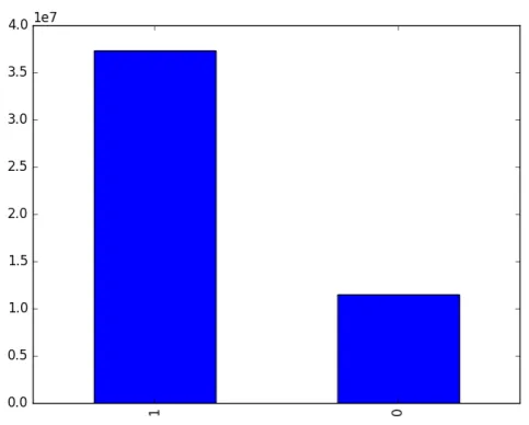
Figure 2.Class distribution (0 - Churn, 1 Not churn)
• Data Preparation : Data cleaning and preparation involves removing missing data and creating binary label that indicates whether a customer will be inactive (not performing any transaction) over the next 3 months. For each customer ID, transactional data for any given month is paired with the inactivity label after the next 3 months period. The resulting dataset consists of 25 sliding windows. Figure2 shows the resulting number of data for each class, where class 1 represents customers that remain active and class 0 represents customers that become inactive.
• Modeling : Data modeling is the process of encapsulating the business and data knowledge into a model that explains the training data. This model is also used to predict unseen labels from a test set. Given the size and complexity of the dataset, in this paper we propose an incremental learning pipeline. The whole pipeline and the different algorithm settings is explained in Section3.
• Evaluation : Performance evaluation is the last stage of the process and involves partitioning the dataset into one or more training and testing datasets. Also, a performance criteria must also be defined in order to assess the validity of the overall results. These metrics and the whole cross-validation results are shown in Section5.
3. Incremental Learning for Predictive Analytics
Obtaining highly informative variables that are neither correlated or missing is difficult, especially in high dimensional settings. This is often the case in most machine learning problems, so dimensionality reduction techniques such as PCA are used to alleviate the construction of such models. However, the cost of projecting the original features into a lower dimensional manifold depends on the size of the data set and therefore cannot be directly used to large scale problems [9]. Although some specific implementations of distributed machine learning techniques for big data analytics exists (e.g. Apache Mahout/Spark1), there is a communication overhead when using a computer cluster. Morover, significant energy savings could be achieved when using an incremental learning strategy for medium-sized datasets in a single computer node [10].
3.1. Incremental PCA
Input data vectors may be very high dimensional but typically lie close to a of very low manifold, meaning that the distribution of the data is heavily constrained. PCA is a linear dimensionality reduction technique that can be obtained through a low-rank factorization operation such as the Singular Value Decomposition (SVD). Given a zero-mean input matrixX ∈ Rn×d, we can write the SVD decomposition as:
ˆ
X=UDVT (1)
where ˆXis the optimal low-rank reconstruction of the original data matrixX,Uis an×rcolumn matrix containing thereigenvectors ofXXT,Vis anotherd×rcolumn matrix with thereigenvectors
ofXTXandDis a square diagonalr×rmatrix.
When large datasets 0 << d << n are taken into consideration, there is a computational bottleneck for the covariance matrix XXT which might eventually not fit into memory. However, it is possible to divide the entire dataset into blocks and process sequentially or in parallel each one of the blocks [11]. Furthermore, this approach is also appealing to the churn prediction problem where data is each block can represent monthly aggregated data and we can use several blocks for parameter estimation and cross-validating results.
AS the name suggests, Incremental Probabilistic Component Analysis (IPCA) incrementally learns a subspace representation of the data from a partial subset of the dataset [3]. The method requires the specification of the number of eigenvalues to be used for the representation (PCA components) but the complete data does not necessarily must fit into memory. This is particularly important for big data analytics when the computation of a full covariance matrix cannot be performed efficiently.
If we now write the input data matrix as the concatenation of two matricesX = [AB]T, we can first compute the SVD ofAto obtain a partial fit ˆA = UDVT and then use this result to compute
[AˆBˆ]T =U0D0V0T. More technical details can be found in [3] 3.2. Stochastic Gradient Decent
Similar to the dimensionality reductions step, we now need to consider algorithms with online learning capabilities. SGD can be used to perform one pass over a data block (mini-batch) and update the model according to the direction of the gradient [2]. The gradient of a functionF(·)with parameter w∈Rr+1is calculated as the sum of a loss functionJ(w) = 1b∑bj J(w;xj,yj)and a regularization term.
The parameterbaccounts for the size of the data block and the loss function can be written as: F(w) =J(w) + α
2kwk
2 (2)
SGD performs partial updates to the unknown parameterwusing the following update rule:
wi=wi−1−ηi∇F(wi) (3)
whereηiis a (possibly non-stationary) learning rule and∇F(w)is the gradient of the empirical
loss function. In the case of logistic regression classifiers, J(w)becomes the negative log-likelihood of the binomial distribution, however when the hinge loss is used the model can also accommodate to a linear SVM with gradient:
∇F(w) =αw−
∑
jwherewimust be scaled with a factor of min{1,√1
λ||w
i||}.
4. Materials and Methods
4.1. Technical Equipment
The technical equipment used has an Intel Xeon processor E5-v2620 with 1Tb storage, two Intel Xeon Phi coprocessors 7120p and 5120p, 32 GB of RAM and the Centos 7 operating system. The programming language wasPython(https://www.python.org),Pandas(http://pandas.pydata.org) was used for data pre-processing and all algorithms were implemented with thescikit-learnlibrary [12].
4.2. Data
The dataset contains information of monthly customer transactions and the churn label was calculated as inactivity in any of the given 19 months. The full dataset contains more than 150 predictors corresponding to different types of transactions with a total size of 23 GB and a total number ofn = data rows. Data pre-processing included : data cleaning (removing null, missing and constant values), transformation (normalization, representing categorical variables as dummy indicator variables, standardization) and label calculation (pairing transactional data with a 3 months ahead churn label). As a result of the data processing task, a total number of 19 labeled data files were produced.
5. Evaluation
To evaluate the performance of the proposed approach we must adjust several design parameters according to an error criteria. Therefore, in order to validate the efficiency of the model parameters, a k-fold cross-validation scheme over different configurations whose performance is measured according to the criteria of accuracyAand precisionPfor classification:
P= |TP|
|TP|+|FP| (5)
A= |TP|+|TN|
|TN|+|FN|+|TP|+|FP| (6)
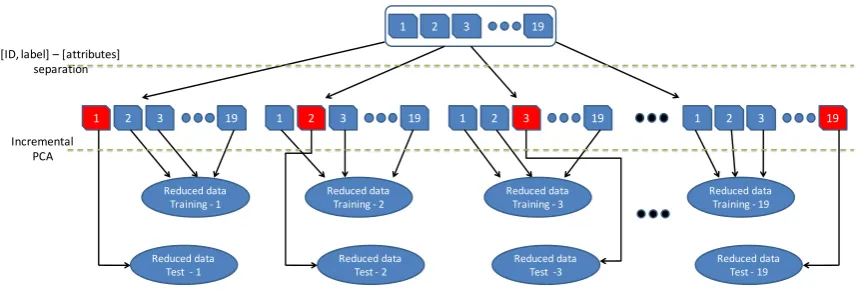
where|TP|i corresponds to the number of true positives, |FP|i the number of false positives, |TN|i the number of true negatives and |FN|i the number of false negatives in the validation set. Figure3shows the k-fold cross-validation scheme.
19 3
2 1
19 3
2
1 1 2 3 19 1 2 3 19 1 2 3 19
Reduced data
Training - 2 Reduced data Training - 3 Reduced data
Training - 1 Reduced data Training - 19
Reduced data
Test - 1 Reduced data Test - 2 Reduced data Test -3 Reduced data Test - 19
[ID, label] – [attributes] separation
Incremental PCA
5.1. Dimensionality Reduction
Dimensionality reduction is first applied through IPCA over thek−1 data blocks. For each fold, IPCA produces two new datasets with reduced dimensionality. The validation block uses the projection matrix obtained from all other blocks in order to create the test dataset for thek−ithblock. The final number of predictors depends on the PCA components, which in turn are the eigenvectors that captures most of the variation of the full dataset.
5.2. Classifier training
SGD uses a loss function J(w)to calculate the gradient of the error, so the classification results are dependent on this function. Typical functions are the Hinge loss, the logarithmic (Log) function and the modified Huber loss. Moreover, the regularization term can also use theL1or L2penalty with different values for theαparameter.
5.3. Grid search cross-validation
The best configuration was determined through a grid search procedure and the performance was measured with the k-fold cross validation procedure. The following configurations were tested:
Table 2.Parameter Setting
Parameter Values
Number of PCA components 5, 10, 20, 30
Loss functions Hinge, Log, Modified Huber
Penalty L1,L2
Regularization constant (α) 0.1, 0.01, 0.001
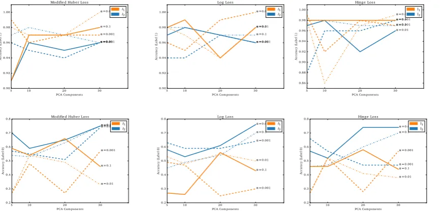
Figure4illustrates the different configuration parameters for thenot churnandchurnclasses, loss functions and different number of PCA components.
5 10 20 30
PCA Com pone nts 0.2 0.3 0.4 0.5 0.6 0.7 0.8 A cc ur ac y (L ab el 0 ) α=0.001 α=0.01 α=0.1 α=0.001 α=0.01 α=0.1 Modifie d Hube r Los s
1 2
5 10 20 30
PCA Com pone nts 0.2 0.3 0.4 0.5 0.6 0.7 0.8 A cc ur ac y (L ab el 0 ) α=0.001 α=0.01 α=0.1 α=0.001 α=0.01 α=0.1 Log Los s
1 2
5 10 20 30
PCA Com pone nts 0.90 0.92 0.94 0.96 0.98 1.00 A cc ur ac y (L ab el 1 ) α=0.001 α=0.01 α=0.1 α=0.001 α=0.01 α=0.1 Modifie d Hube r Los s
1 2
5 10 20 30
PCA Com pone nts 0.90 0.92 0.94 0.96 0.98 1.00 A cc ur ac y (L ab el 1 ) α=0.001 α=0.01 α=0.1 α=0.001 α=0.01 α=0.1 Log Los s
1 2
5 10 20 30
PCA Com pone nts 0.86 0.88 0.90 0.92 0.94 0.96 0.98 1.00 A cc ur ac y (L ab el 1 ) α=0.001 α=0.01 α=0.1 α=0.001 α=0.01 α=0.1 Hing e Los s
l1 l2
5 10 20 30
PCA Com pone nts 0.2 0.3 0.4 0.5 0.6 0.7 0.8 A cc ur ac y (L ab el 0 ) α=0.001 α=0.01 α=0.1 α=0.001 α=0.01 α=0.1 Hing e Los s
l1 l2
Figure 4.Cross-validation results using different number of PCA components and model parameters. TheHingeloss function shows improved performance in terms of accuracy in training when compared
to theLogandModified Huberloss functions. Also, training the model with the L2 penalty and the
5.4. Model Evaluation
The selected configuration is based on the best performance for both classes and weighting samples according to the minority class.
Table 3.Selected parameter setting
Parameter Value
IPCA number of components 30 Loss function Hinge
Penalty L2
Regularization constant (α) 0.01
Learning rate Optimal
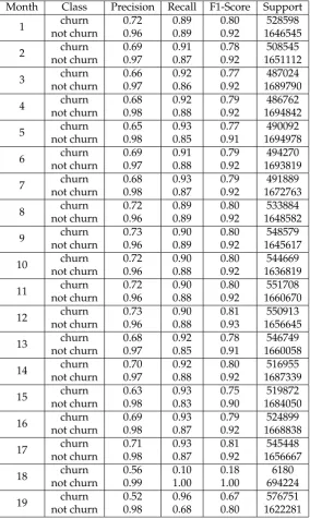
Usingtheselectedmodelparameters,K-foldcross-validationaccuracyandprecisionresultsare showninTable4:
Table 4.Monthly prediction results
Month Class Precision Recall F1-Score Support
1 churn 0.72 0.89 0.80 528598
not churn 0.96 0.89 0.92 1646545
2 churn 0.69 0.91 0.78 508545
not churn 0.97 0.87 0.92 1651112
3 churn 0.66 0.92 0.77 487024
not churn 0.97 0.86 0.92 1689790
4 churn 0.68 0.92 0.79 486762
not churn 0.98 0.88 0.92 1694842
5 churn 0.65 0.93 0.77 490092
not churn 0.98 0.85 0.91 1694978
6 churn 0.69 0.91 0.79 494270
not churn 0.97 0.88 0.92 1693819
7 churn 0.68 0.93 0.79 491889
not churn 0.98 0.87 0.92 1672763
8 churn 0.72 0.89 0.80 533884
not churn 0.96 0.89 0.92 1648582
9 churn 0.73 0.90 0.80 548579
not churn 0.96 0.89 0.92 1645617
10 churn 0.72 0.90 0.80 544669
not churn 0.96 0.88 0.92 1636819
11 churn 0.72 0.90 0.80 551708
not churn 0.96 0.88 0.92 1660670
12 churn 0.73 0.90 0.81 550913
not churn 0.96 0.88 0.93 1656645
13 churn 0.68 0.92 0.78 546749
not churn 0.97 0.85 0.91 1660058
14 churn 0.70 0.92 0.80 516955
not churn 0.97 0.88 0.92 1687339
15 churn 0.63 0.93 0.75 519872
not churn 0.98 0.83 0.90 1684050
16 churn 0.69 0.93 0.79 524899
not churn 0.98 0.87 0.92 1668838
17 churn 0.71 0.93 0.81 545448
not churn 0.98 0.87 0.92 1656667
18 churn 0.56 0.10 0.18 6180
not churn 0.99 1.00 1.00 694224
19 churn 0.52 0.96 0.67 576751
6. Conclusions
An incremental learning approach for large scale churn prediction has been presented. The proposed approach uses an incremental version of PCA that can efficiently compute eigenvalues of big matrices, so it can be used when the size of the dataset does not fit into memory. Furthermore, a fully incremental learning model was also delivered using SGD, which performs on line training using data batches. The proposed approach was evaluated with several months of data and each month was used as a hold-out sample for validation, while the rest of the data is used to incrementally train the model. Although the model was built using a large sample, the overall results show an average of 64% of success for the churn class, which is still lower than previously reported results using other learning techniques (such as non-linear SVM). Because of the difficulty of training more complex learning models at a large scale, it is still difficult to compare these results, so accelerating training and data pre-processing should be done in order to perform feature engineering for improving the classification rates.
Acknowledgment
This paper has been funded by CONICYT/FONDECYT/INICIACION 11140598.
Bibliography
1. T. Vafeiadis, K.I. Diamantaras, G. Sarigiannidis, and K.Ch. Chatzisavvas. A comparison of machine learning
techniques for customer churn prediction. Simulation Modelling Practice and Theory, 55:1 – 9, 2015.
2. K. P. Murphy. Machine learning: a probabilistic perspective. MIT press, 2012.
3. D. A. Ross, J. Lim, R-S. Lin, and M-H. Yang. Incremental learning for robust visual tracking. International
Journal of Computer Vision, 77(1-3):125–141, 2008.
4. B. Huang, M. Tahar Kechadi, and B. Buckley. Customer churn prediction in telecommunications. Expert
Systems with Applications, 39(1):1414 – 1425, 2012.
5. X. Yu, S. Guo, J. Guo, and X. Huang. An extended support vector machine forecasting framework for
customer churn in e-commerce. Expert Systems with Applications, 38(3):1425 – 1430, 2011.
6. F. Huang, Y .and Zhu, M. Yuan, K. Deng, Ya. Li, B. Ni, W. Dai, Q. Yang, and J. Zeng. Telco churn prediction
with big data. InProceedings of the 2015 ACM SIGMOD International Conference on Management of Data, pages
607–618. ACM, 2015.
7. C. Croux A. Lemmens. Bagging and boosting classification trees to predict churn. Journal of Marketing
Research, 43(2):276–286, 2006.
8. E. W. Ngai, L. Xiu, and D. CK. Chau. Application of data mining techniques in customer relationship
management: A literature review and classification. Expert systems with applications, 36(2):2592–2602, 2009.
9. N. Kettaneh, A. Berglund, and S. Wold. Pca and pls with very large data sets.Computational Statistics & Data
Analysis, 48(1):69–85, 2005.
10. H Zhao and J. Canny. Butterfly mixing: Accelerating incremental-update algorithms on clusters. InSIAM
Conf. on Data Mining. SIAM, 2013.
11. T. Elgamal and M. Hefeeda. Analysis of pca algorithms in distributed environments. arXiv preprint
arXiv:1503.05214, 2015.
12. F. Pedregosa, G. Varoquaux, A. Gramfort, V. Michel, B. Thirion, O. Grisel, M. Blondel, P. Prettenhofer, R. Weiss, V. Dubourg, J. Vanderplas, A. Passos, D. Cournapeau, M. Brucher, M. Perrot, and E. Duchesnay.
Scikit-learn: Machine learning in Python. Journal of Machine Learning Research, 12:2825–2830, 2011.
c
2016 by the authors; licenseePreprints, Basel, Switzerland. This article is an open access