www.earth-syst-dynam.net/3/263/2012/ doi:10.5194/esd-3-263-2012
© Author(s) 2012. CC Attribution 3.0 License.
Earth System
Dynamics
Spatio-temporal analysis of the urban–rural gradient structure:
an application in a Mediterranean mountainous landscape
(Serra San Bruno, Italy)
G. Modica1, M. Vizzari2, M. Pollino3, C. R. Fichera1, P. Zoccali1, and S. Di Fazio1
1Mediterranea University of Reggio Calabria, Department of Agroforestry and Environmental Sciences and Technologies
(DiSTAfA), loc. Feo di Vito c/o Facolt`a di Agraria, 89122 Reggio Calabria, Italy
2Department of Man and Territory, University of Perugia, Borgo XX Giugno 74, 06121 Perugia, Italy
3ENEA – National Agency for New Technologies, Energy and Sustainable Economic Development, “Earth Observations and
Analyses” Lab (UTMEA-TER), Casaccia Research Centre – Via Anguillarese 301, 00123 Rome, Italy
Correspondence to: G. Modica ([email protected])
Received: 2 August 2012 – Published in Earth Syst. Dynam. Discuss.: 20 August 2012 Revised: 20 November 2012 – Accepted: 25 November 2012 – Published: 19 December 2012
Abstract. The most recent and significant transformations of European landscapes have occurred as a consequence of a series of diffused, varied and often connected phenom-ena: urban growth and sprawl, agricultural intensification in the most suitable areas and agricultural abandonment in marginal areas. These phenomena can affect dramatically ecosystems’ structure and functioning, since certain modi-fications cause landscape fragmentation while others tend to increase homogeneity. Thus, a thorough comprehension of the evolution trends of landscapes, in particular those linked to urban-rural relations, is crucial for a sustainable landscape planning.
In this framework, the main objectives of the present pa-per are: (a) to investigate Land Use/Land Cover (LULC) transformations and dynamics that occurred over the period 1955–2006 in the municipality of Serra San Bruno (Calabria, Italy), an area particularly representative of the Mediter-ranean mountainous landscape; (b) to compare the settle-ment growth with the urban planning tools in charge in the study area; (c) to examine the relationship between urban– rural gradient, landscape metrics, demographic and physical variables; (d) to investigate the evolution of urban–rural gra-dient composition and configuration along significant axes of landscape changes.
Data with a high level of detail (minimum mapping unit 0.2 ha) were obtained through the digitisation of historical aerial photographs and digital orthophotos identifying LULC
classes according to the Corine Land Cover legend. The vestigated period was divided into four significant time in-tervals, which were specifically analysed to detect LULC changes.
Differently from previous studies, in the present research the spatio-temporal analysis of urban–rural gradient was per-formed through three subsequent steps: (1) kernel density analysis of settlements; (2) analysis of landscape structure by means of metrics calculated using a moving window method; (3) analysis of composition and configuration of the urban– rural gradient within three landscape profiles located along significant axes of LULC change.
The use of thematic overlays and transition matrices en-abled a precise identification of the LULC changes that had taken place over the examined period. As a result, a de-tailed description and mapping of the landscape dynamics were obtained. Furthermore, landscape profiling technique, using continuous data, allowed an innovative and valuable approach for analysing and interpreting urban–rural gradient structure over space and time.
1 Introduction
a corresponding increase in industrial activities and agri-cultural intensity. The consequent transformations of urban-rural systems are one of the most important types of Land Use/Land Cover (LULC) changes, since they are widespread all over the world and often determine negative effects on ecosystem functionality. Although most of the actions lead-ing to LULC changes have a local origin, nevertheless their speed, extension and intensity bring about important global implications, in particular in carbon (Foley et al., 2005) and water cycles (Turner and Rusher, 1988). Moreover, LULC changes can dramatically affect the structure and functioning of ecosystems (Defries et al., 2004; Vitousek, 1997), since certain modifications cause landscape fragmentation while others tend to increase homogeneity (Forman, 1995; Farina, 1998). Their analysis is one of the main research topics of ecology (Braimoh, 2006) and landscape ecology (Wu and Hobbs, 2002). Therefore, the evaluation of LULC present status and trends of change can provide crucial ecological information for science-oriented resource management and policy making, in relation to a wide range of human activi-ties (Cihlar, 2000).
Urbanisation is a complex diffusion process that is dra-matically spreading and variously affecting rural landscape at different spatial scales. The urbanisation process en-tails the transformation of landscapes, characterised by ru-ral lifestyles, into urban ones and determines functional and structural changes, thus creating new landscape patterns (Antrop, 2000). It can give rise to the most dramatic form of irreversible land modification (Luck and Wu, 2002) which poses threats on biodiversity and landscape integrity.
Urban sprawl is an inherently dynamic spatial phe-nomenon defined as a specific form of urban develop-ment with low density, dispersed spatial pattern and auto-dependent as well as environmentally and socially impacting characteristics (Hasse and Lathrop, 2003), which can be con-sidered as one of the main challenges in spatial planning in the 21st century (Poelmans and Van Rompaey, 2009). The term “sprawl” is often used to describe the awareness of an unsuitable development, of a disordered growth of urban ar-eas (Sudhira et al., 2004). Taking into account its efficiency in terms of hectares of new development in relation to the number of people supported, sprawl can be considered as an “inefficient new urban growth” (Hasse and Lathrop, 2003). Thus, urban sprawl is the consequence of many individual decisions and some of its causes are population growth, eco-nomic issues and proximity to resources and basic facilities (Hoffhine Wilson et al., 2003).
Especially in the Mediterranean area, the urbanisation pro-cess is still ongoing with significant effects in landscape frag-mentation and in loss of ecosystem services (EEA, 2011). Historically, urban development and agriculture have acted as counterposed activities in competition for the use of land: the expansion of cities has typically taken place on for-mer agricultural lands (Hidding et al., 2000; Perella et al., 2010; Perchinunno et al., 2012). Just to mention a few data,
between 1990 and 2000, the amount of land consumed by urban areas and associated infrastructure throughout Europe was about 800 km2yr−1 (EEA, 2006b). In Italy, in
particu-lar, an increase in urban pressure on the countryside can still be observed, owing to land renting and displacement of cer-tain typical urban functions outside the cities (Murgante and Danese, 2011). This trend is a reversal of the demographic and territorial dynamics occurred during the period immedi-ately following the Second World War and has resulted in the progressive urbanisation of rural areas; in a general in-crease in the number of inhabitants in the peri-urban belts; and in a decrease in resident population in towns (Alberti et al., 1994).
The Mediterranean area is one of the most significantly altered hotspots on Earth (Myers et al., 2000). Here, the widespread agricultural lands, evergreen woodlands and maquis shrublands are the result of anthropogenic distur-bances occurred over centuries or even millennia (Blondel, 2006). The most recent and significant LULC changes have occurred as a consequence of a series of diffused, varied and often connected phenomena: urban sprawl; agricultural in-tensification in the most suitable areas and agricultural aban-donment in marginal areas; more frequent and more intense summer forest fires; and rapid expansion of tourism activities and infrastructures, mainly along the coasts (Antrop, 2004; EEA, 2006b, 2011; Neri et al., 2010).
Owing to these continuous anthropic pressures and ac-cording to the different physical and climate conditions, fur-ther research is needed to monitor and analyse, in quanti-tative and qualiquanti-tative terms, ongoing LULC changes (EEA, 2006b, 2011; Fusco Girard and De Toro, 2007; Fichera et al., 2011) and trends of rural gradients. Data on urban-rural transformations are a valuable source of information in understanding the methods and the effects of urban land-scape changes and trends. As a consequence, they can in-fluence the formulation of guidelines and policies to address future growth as well as to put into practice urban greenspace protection.
The gradient approach in landscape ecological analysis al-lows for a more realistic representation of landscape hetero-geneity by not presupposing schematisations and discreti-sations of the natural and anthropic environment (McGari-gal and Chusman, 2005). Urbanisation can be considered as a particular environmental gradient that produces modifica-tions on the structures and funcmodifica-tions of the ecological sys-tem (McDonnell and Hahs, 2008). Thus, also the traditional urban-rural dichotomy can be thought as a landscape gradi-ent, whose representation mutates depending on the natural and anthropic variables taken into account and to the spatio-temporal scale adopted for the analysis.
LANDSCAPE GRADIENTS
Aerial photos, Satellite images,
GCPs
Image Georeferentiation, Orthorectification, Processing and Classification
Digital cartography
Data extraction and conversion
General Master Plan (GMP)
Vectorialisation, Data extraction and
conversion
LULC transition matrices KDE of main landscape components
INTERMEDIATE MAPS
Interpretation of landscape dynamics
LULC MAPS SETTLEMENTM
APS
GMP VECTORIALISED
URBAN-RURAL TRANSFORMATIONS
LANDSCAPE STRUCTURE
GMP ANALYSIS Landscape metrics analysis
Urban-rural gradient
structure GMP effectiveness
DA
TA
PROCESSING
RESUL
T
S
DA
TA
ANAL
YSIS
FINAL LANDSCAPE MAPS
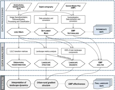
Fig. 1. Flow-chart showing the main methodological phases of the research framework.
2006; McDonnell and Hahs, 2008; Yang et al., 2010; Vizzari, 2011a).
One effective method for representing and analysing the urban–rural gradient and the urban sprawl is using Kernel Density Estimation (KDE) techniques applied on locations of buildings (Torrens and Alberti, 2000; Vizzari, 2011a). Den-sity analysis takes measured quantities associated with point data and spreads them across the landscape to produce a con-tinuous surface. Unlike simple density estimation, KDE pro-duces smoother surfaces that are more representative of land-scape gradients (Vizzari, 2011b). In KDE, a moving win-dow is superimposed over a grid of locations and the den-sity of events is estimated at each location using a distance-weighted function, with the degree of smoothing controlled by the kernel bandwidth (Gatrell et al., 1996). Since the first study on KDE proposed by Fix and Hodges (Silverman and Jones, 1989), many improvements of this smoothing tech-nique have been developed by several authors, particularly within spatial analysis applications (see Danese et al., 2008 and references therein).
With the aim to explore the relationships between ecosys-tem processes and services and landscape patterns, a valu-able source of information can be obtained from using land-scape metrics. According to Botequilha Leit˜ao et al. (2006), landscape is the optimal scale for sustainable land planning,
considering that landscapes are usually large enough and in-trinsically consistent with the scale of human perception, decision-making and physical management (Forman, 1995; Botequilha Leit˜ao and Ahern, 2002). Landscape metrics are useful tools in mapping and quantifying spatial LULC char-acteristics and temporal variation (Cushman et al., 2008) as well as in understanding the process of urbanisation and its ecological effect at landscape level (Sudhira et al., 2004; Peng et al., 2010). Plenty of metrics can be efficiently calcu-lated using specific software packages, such as FRAGSTATS (McGarigal et al., 2012), and, despite all their conceptual flaws, risks of improper use and well-known limitations (Cushman et al., 2008; Li and Wu, 2004), they continue to be widely used in quantitative landscape ecology studies aimed at the analysis of landscape structure. Landscape metrics find a very effective application in the analysis of urban to rural gradient composition and configuration (e.g. Luck and Wu, 2002; Hahs and McDonnell, 2006; Weng, 2007; Yang et al., 2010).
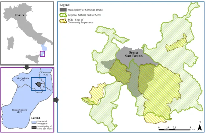
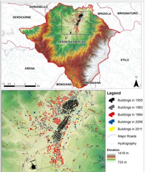
Fig. 2. Map showing the geographical location of the study area. In the blue box, the boundaries of protected areas falling in the territory of
Serra San Bruno municipality are mapped.
examine the relationship between urban–rural gradient, land-scape metrics and demographic and physical variables; (d) to investigate the evolution of urban–rural gradient composi-tion and configuracomposi-tion along significant axes of landscape changes.
Unlike previous studies (e.g. Luck and Wu, 2002; Hahs and McDonnell, 2006), in this research, the spatio-temporal analysis of urban–rural gradient was performed through three steps: (1) kernel density analysis of settlements; (2) analysis of landscape structure by means of metrics calculated using a moving window method; (3) analysis of the gradient com-position and configuration within three landscape profiles lo-cated along significant axes of LULC change.
2 Materials and methods
2.1 Study area
The research was carried out in the territory of the munici-pality of Serra San Bruno (Fig. 2), located in Serre Vibonesi, a mountainous area of Calabria (a region of Southern Italy) presenting many heritage resources of great natural, historic and architectural interest.
The municipality has an area of circa 4000 ha, a resi-dential density of 174.5 inhab. km−2 and is situated at an average altitude of 980 m a.s.l. Centuries-old woods, char-acterised by the prevalence of chestnut (Castanea sativa Miller), beech (Fagus sylvatica L.) and silver fir (Abies alba Miller subsp. apennina Brullo, Scelsi and Spampinato) pop-ulations, highlight the intrinsic suitability of this land for forestry production. Starting from the 1950s, reforestation
has been practised by planting first conifers, such as the European black pine (Pinus laricio Poiret) and fir-douglas (Pseudotsuga menziesii (Mirb.) Franco), and then broad-leaved trees, such as chestnut. According to Quezel and Medail (2003), EEA (2006a), Blasi et al. (2010) and Mer-curio (2010), the landscape analysed can be classified as Mediterranean.
For centuries, the forests were owned by the Charterhouse of Serra San Bruno, which was founded by St. Bruno of Cologne in the 11th century. They were managed efficiently and sensitively according to the methods of the Carthusian monks. Count Roger II gave St. Bruno of Cologne the ter-ritories of Serre Vibonesi plateau to build his hermitage, the Charterhouse of Santo Stefano del Bosco, second Carthusian monastery in Europe after the one in Grenoble (France). The high environmental value of this area motivated the institu-tion of two Nainstitu-tional Natural Reserves (now SCIs – Sites of Community Importance – of the Natura 2000 network, the centrepiece of the EU’s nature and biodiversity policy) and of the Regional Natural Park of Serre in 2004. The local in-dustrial archaeology heritage is also very significant. It is re-lated to the utilisation of water and wood as energy sources and dates back to the time of the Bourbon rule in Calabria (XVIII–XIX centuries). Also worth mentioning is that in the same area there are many historic monastic complexes, some of which are still inhabited by the original religious orders, either Catholic or Greek Orthodox.
depopulation and many traditional economic activities, such as charcoal production, became weak and went through peri-ods of crisis. Recently, the development of forms of tourism, based on the valorisation of the rich cultural and natural resources, has been of some help in sustaining the local economy. Tourists search for high landscape quality, which should be improved through sensitive landscape planning based on accurate monitoring of the dynamics characteris-ing land use (Selicato et al., 2012). This is also needed for the maintenance of the environmental balance of these areas, which are particularly fragile since they are exposed to rele-vant hydrogeologic risk (the last catastrophic flood occurred in 1935, causing death and destruction).
2.2 Data processing
For the aims of this research, observation covered a period of intense and radical transformation of the Italian economic, cultural and territorial assets, ranging from the end of Sec-ond World War to present years. The first step towards the detection of LULC changes was the acquisition of all the rel-evant LULC maps referred to the period under investigation. LULC changes were analysed using aerial photographs from the Italian Military Geography Institute (IGMI), for years 1955 and 1983, and digital georeferenced orthophotos from the National Geoportal (NG) of the Italian Ministry of the Environment, for years 1994 and 2006. All the aerial pho-tographs were georeferenced by using 20–30 Ground Con-trol Points (GCP) and orthorectified by using a Digital El-evation Model (DEM) with 10 m×10 m of spatial resolu-tion. Four datasets with a spatial resolution of 1.37 m and an RMSE (Root Mean Square Error) of less than 6.5 m were produced. A set of 1998 orthophotos, a 1 : 10 000 numerical topographic map and the DEM were used as reference mate-rial (for further details see Di Fazio et al., 2011).
In order to produce settlement-strata to perform the ur-ban gradient analysis for the period under investigation, the buildings in the study area were digitised according to all the time intervals defined. In addition, a Worldview-2 scene for year 2011 was processed (Updike and Comp, 2010) in view of extracting the settlement stratum. To this end, an RGB colour orthophoto was produced from the original multispec-tral image that had been georeferenced and orthorectified, us-ing 30 GCP and the available DEM, and then pan-sharpened. A Subtractive Resolution Merge technique was used for the purpose.
2.3 Analysis of the landscape mosaic evolution
2.3.1 LULC mapping changes
LULC maps are commonly produced either by aerial visual interpretation or by classification of remotely sensed images. Definitely, photo-interpretation requires skilled analysts, is a time-consuming technique and is subjective, considering
Fig. 3. LULC maps of the study area for all years under
investiga-tion and graphical representainvestiga-tion according to the LULC class types composition.
the high degree of operator control. Nevertheless, it is still widely used and considered as a useful source of informa-tion in studies focussing on landscape pattern analysis (Zhou et al., 2009) and landscape change (Ode et al., 2010), owing to the scarcity, if not lack, of historic satellite imagery related to the years before the 1970s. In this research, LULC map-ping was conducted by visual photointerpretation, thanks to the availability of aerial photographs referring to the period investigated and characterised by good frequency and high spatial resolution.
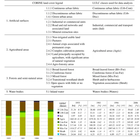
Table 1. Correspondence between CORINE legend nomenclature and LULC classes used for detecting LULC changes. In brackets, the
symbols utilised in the text and in following figures.
CORINE land cover legend LULC classes used for data analysis
1. Artificial surfaces
1.1.1 Continuous urban fabric Continuous urban fabric (Urb-Cont)
1.1.2 Discontinuous urban fabric Discontinuous urban fabric
(Urb-1.4.1 Green urban areas Disc)
1.2.1 Industrial or commercial units
1.2.2 Road and rail networks and Industrial, commercial and transport
associated land units (Ind)
1.3.1 Mineral extraction sites
2. Agricultural areas
2.1.1 Non-irrigated arable land 2.3.1 Pastures
2.4.1 Annual crops associated with permanent crops
2.4.2 Complex cultivation patterns Agricultural areas (Agric) 2.4.3 Land principally occupied by
agriculture, with significant areas of natural vegetation
2.4.4 Agro-forestry areas
3. Forests and semi-natural areas
3.1.1 Broad-leaved forest Broad-leaved forest (Blv-For)
3.1.2 Coniferous forest Coniferous forest (Con-For)
3.1.3 Mixed forest Mixed forest (Mix-For)
3.2.4 Transitional woodland shrub Shrub and/or herbaceous 3.3. Open spaces with little or no Vegetation associations (Shrub)
vegetation
5. Water bodies 5.1 Inland water Waters bodies (Waters)
Fig. 4. Landscape composition of the study area in the four time intervals investigated, based on the 9 LULC class types. Data in [ha] and in
[%]. In addition, for each LULC class the NP (Number of Patches) is shown.
legend. The original 44 LULC classes at level III detail were aggregated in 9 classes (Table 1) so as to interpret changes as
change types (Di Fazio et al., 2011).
The spatial comparison of LULC vector maps was per-formed for the years 1955, 1983, 1994 and 2006 by means of a post-classification comparison technique that could pro-vide a complete matrix of change directions (Lu et al., 2004). It is a type of change detection obtained through a cross-tabulation analysis which enables to highlight the changes occurred in time both in qualitative terms, by showing them
directly on the map, and in quantitative terms, by allowing to calculate the total areal extent of land use change occurred at different times. Relative and absolute changes for each of the 9 LULC types were calculated from 9x9 transition ma-trices (or cross-tabulation mama-trices). The transition mama-trices were built for the time intervalt1tot2, wherein rows display
the categories of time 1 and columns display the categories of time 2. While row vectors show the evolution of a land use type in the periodt1–t2, column vectors show the land
2006
1955 Urb-Cont Urb-Disc Ind Agric Con-For Blv-For Mix-For Shrub Waters Sum 1955
Urb-Cont 30.98 - - - 0.36 31.34
Urb-Disc - 4.48 - - - 4.48
Ind - - 1.97 - - - 1.97
Agric 24.68 72.21 27.39 789.43 87.51 484.82 133.14 41.07 2.92 1663.18
Con-For - - - - 12.86 0.36 39.90 1.20 - 54.38
Blv-For - 0.74 - 29.28 1.02 160.78 25.29 0.33 - 217.44
Mix-For 0.27 - 0.75 8.82 138.18 18.10 1749.21 2.93 - 1918.27
Shrub 2.76 0.28 - 14.72 5.48 50.99 42.44 5.25 - 121.91
Waters 1.07 2.76 0.25 4.98 - 10.41 0.78 0.76 3.61 24.64
Sum 2006 59.76 80.47 30.41 847.24 245.05 725.46 1990.77 51.55 6.89 4037.60
Fig. 5. Transition matrix for the Time period 1955–2006.
generated at timet2. The data of the main diagonal, shown
in bold, indicate the area of LULC persistence. In this pa-per, changes detected in the period 1955–2006 are reported (Fig. 5). For further information about the results of the inter-mediate time interval analysis (1955–1983, 1983–1994 and 1994–2006), please refer to Di Fazio et al. (2011).
2.3.2 Landscape metrics analysis at class and landscape levels
With the aim to better understand and describe the expand-ing footprints of residential and urban areas, the landscape composition and configuration of the study region was in-vestigated by using landscape metrics. When applying spa-tial metrics, the spaspa-tial unit used is called patch, defined as a relatively homogeneous area that differs from its surround-ings (Forman, 1995). The basis of the spatial metric calcu-lation is a thematic map (either in vector or raster format) representing a landscape composed of spatial patches cate-gorised in different patch classes. Landscape metrics can be defined as quantitative and aggregate measurements based on a categorical, patch-based representation of a landscape showing spatial heterogeneity at a specific scale and reso-lution (Herold et al., 2003, 2005) and represent one of the key factors in landscape ecological research (Uuemaa et al., 2009) and in landscape planning. According to several au-thors (e.g. Gustafson, 1998; Herold et al., 2003, 2005; Seto and Fragkias, 2005; Aguilera et al., 2011), the term spatial
metrics relates to the characterisation of urban forms as such,
while the term landscape metrics explicitly links to ecolog-ical functions. A major value of landscape metrics lies in their usefulness for comparing alternative landscape configu-rations, for example in evaluating the same landscape at dif-ferent time periods (Gustafson, 1998).
For the purpose of this research, and according to Cush-man et al. (2008), a set of limited-number landscape metrics with a valuable meaning in analysing landscape composition
and configuration was selected, both at class and landscape level and for all the time intervals defined (Fig. 6 gives a short explanation for each of them). The land-use datasets (1955, 1983, 1994 and 2006) were first converted into grid format (pixel size 10 m×10 m) in order to perform synoptic metric analyses and further analyses using the FRAGSTATS pack-age v. 4.0 (McGarigal et al., 2012).
2.4 Analysis of urban planning tools
This subsequent step of the research activities was aimed to study the current urban planning tools of Serra San Bruno from their implementation until today, and to assess their stages of development. The General Master Plan (GMP) was adopted as a municipal planning tool in 1997 and is now be-ing updated so as to help direct new urbanisation processes towards areas that are not intended for agricultural and for-est use. The analyses carried out were also aimed to analyse LULC maps focussing on built-up areas, in order to evalu-ate their importance and role in shaping the character of the town. The processing of the above-mentioned thematic maps was performed to examine urban planning effectiveness and to provide a base to suggest recommendations for future im-provements and support management tasks.
In this framework, GIS tools were used by exploiting their capability to support spatial analysis and give suggestions to planners and policy makers. One of the major benefits of this approach is that highly visual and interactive modelling and analysis can be performed. The existing raster map, which represents the GMP of Serra San Bruno, was transformed into vector format by means of semiautomatic editing. The new layer produced represents the zoning of the town ac-cording to the indication of the GMP and includes 16 differ-ent land use categories (Inner city, Completion, Expansion, Public area, Green areas, etc.) as shown in Fig. 7.
Landscape metrics Range Units Description Years
1955 1983 1994 2006
Number of Patches (NP) ≥ 1, without limit None Equals the number of patches in the landscape. 76 122 167 179
Patch Density (PD) constrained ≥ 0, by cell size
Number per 100 hectares
Equals the number of patches of the corresponding patch type divided by
total landscape area (m2). 1.88 3.02 4.14 4.43
Edge Density (ED) ≥ 0, without limit Meters per hectare Equals the sum of the lengths (m) of all edge segments involving the corresponding patch type, divided by the total landscape area (m2). 34.43 54.46 58.37 66.27
Percentage of
Like Adjacencies (PLADJ) 0 ൊ100 Percent
Equals the number of like adjacencies involving the focal class, divided
by the total number of cell adjacencies involving the focal class. 98.03 97.03 96.83 96.44
Interspersion and
Juxtaposition Index (IJI) 0÷100 Percent
Equals minus the sum of the length (m) of each unique edge type divided by the total landscape edge (m), multiplied by the logarithm of the same quantity, summed over each unique edge type; divided by the logarithm of the number of patch types times the number of patch types minus 1 divided by 2.
57.93 59.31 61.53 61.23
Shannon's Diversity Index (SHDI)
≥ 0, without
limit None
Equals minus the sum, across all patch types, of the proportional
abundance of each patch type multiplied by that proportion. 1.12 1.29 1.34 1.40
Simpson's Diversity Index
(SIDI) 0÷1 None
Equals 1 minus the sum, across all patch types, of the proportional
abundance of each patch type squared. 0.60 0.64 0.65 0.68
Fig. 6. Description of landscape metrics (based on McGarigal et al., 2012) and their values obtained at landscape level for all time intervals
under investigation.
Fig. 7. Analysis of the General Master Plan adopted in 1997, in
force until 2007 and currently being updated.
like Serra San Bruno. The goal of this analysis was to cal-culate the effectiveness of zoning: the degree of success of the 1997 GMP was evaluated by taking into account both its indications and built-up expansion in the last 15 yr. To this end, a geoprocessing approach was pursued through a GIS overlay of built-up evolution (1994, 2006 and 2011), zoning layer and LULC maps. In compliance with previous stud-ies (e.g. Luck and Wu, 2002; Hahs and McDonnell, 2006), the integration of demographic and physical data, during this phase of the analysis, allowed a better comprehension of the urban–rural gradient evolution.
2.5 Urban–rural gradient analysis
In this particular application, urban–rural gradient analysis was performed through three consecutive steps: (1) land-scape metrics calculation within FRAGSTAT software us-ing a movus-ing window analysis; (2) Settlement Density In-dex (SDI) calculation by means of Kernel Density Estimation (KDE); (3) landscape gradients analysis along three signifi-cant axes of LULC changes.
2.5.1 Landscape metrics via moving window analysis
Legend Simpson s Diversity Index
1983
2006 1994
1955
Fig. 8. Simpson’s Diversity Index (SIDI) calculated in FRAGSTATS environment using the moving window method.
metrics calculated as well as to improve the smoothing effect on produced maps. According to previous studies, carried out for study areas comparable with the one presented in this pa-per for both extension and geometric data resolution, results with a 500 m radius window have proved to be more effective in revealing landscape metrics fluctuations (Kong and Nak-agoshi, 2006; Kong et al., 2012). Furthermore, this window size is equal to the one adopted for the SDI implementation described below, so as to produce relevant landscape metrics spatially comparable with the SDI analysis. Considering that FRAGSTATS gives negative values for cells located close to the edge and not fully contained within the window of the in-put grid (McGarigal et al., 2012), a buffer area (or expansion strip, as it is referred to by McGarigal et al., 2012), equal to the radius of the window size (500 m), was first defined along the outline of the input LULC raster grid in order to minimise the boundary effect. The maps obtained with this procedure show the spatial distribution of landscape structure based on the results of the selected metrics.
Several landscape metrics were tested across the study-area in order to better understand landscape change patterns and evolution trends. In this phase of the research, a set of three metrics with moving window analysis were selected, owing to their efficacy in supporting the analysis of urban– rural gradient: Agricultural percentage of landscape (A-PLAND), Natural percentage of landscape (N-PLAND) and Simpson’s Diversity Index (SIDI, Simpson, 1949) (Fig. 8). The first two indices indicate, for every pixel, the propor-tion of the circular window (centred on the pixel itself) oc-cupied by agricultural land uses (mostly sowable lands) and by natural land covers (grasslands, woodlands, etc.), respec-tively. Furthermore, in conjunction with SDI, they support the analysis of the main components influencing the urban– rural gradient composition. SIDI has an interpretation that is much more intuitive than Shannon’s index (SHDI, Shannon
and Weaver, 1949) and less sensitive to the presence of rare types (Nagendra, 2002; McGarigal et al., 2012). Like SHDI, also SIDI has been widely used in several studies for rep-resenting landscape diversity changing in space and time. Ranging from 0 (low complexity: only one patch dominates the scene) and 1 (high complexity: all patch types are evenly distributed), Simpson’s index defines the probability that two equal-sized and randomly selected sub-units of landscape belong to different class types. This diversity index com-bines evaluations of richness and evenness. It increases with the increase of the number of class types (richness) and/or when proportional distribution of area among class types be-comes more equitable. In turn, since it reflects the patch abundance and heterogeneity in landscapes, the SIDI index can be used to assess landscape diversity. To this end, how-ever, it is necessary to take into account evidence given by Nagendra (2002) on the need for caution when using SHDI and SDI in assessing landscape diversity.
2.5.2 Settlement density analysis using kernel density estimation
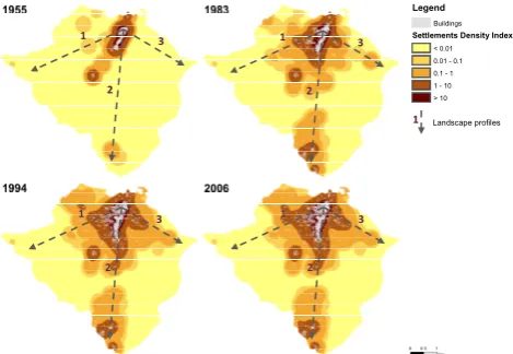
common method for the definition of this parameter (Gatrell et al., 1996; Lloyd, 2007). In this study, after different tests (bandwidths of 100, 250, 500, 750, 1000 m), it was finally de-cided to adopt a bandwidth of 500 m in the analysis of build-ings density at the working scale. Thus, KDE was performed within SAGA GIS (B¨ohner et al., 2006) using a quartic func-tion, a cell size of 50 m and the area occupied by each build-ing as intensity parameter. Considerbuild-ing the method of calcu-lation, the calculated SDI expresses settlement concentration in a given area as the surface occupied by settlements over the territorial surface (Fig. 9). As a consequence, it gives a sim-plified but reliable representation of the gradient of urban-isation: it assumes maximum values in the central portions of more extensive urban areas and progressively decreases when moving towards less urbanised areas. The same fig-ures show the localisation of the landscape profiles described hereinafter.
2.5.3 Landscape gradients analysis through linear profiles
The overall analysis of the urban–rural gradient of the area was performed developing a landscape profiling technique: three different cross-sections (profiles) were located along the main urban development direction with their starting point in the most urbanised area (maximum SDI) (Fig. 9). Using GIS overlay technique, every section was intersected with the four indicator maps of SDI, A-PLAND, N-PLAND and SIDI. The tabular results of the intersection were plotted on different graphs showing the composition and the config-uration of the urban–rural gradient along the three landscape cross-sections and its progressive transformations.
3 Results and discussions
3.1 Urban–rural transformations
During the period examined, all of the stages of land transfor-mations (sensu Forman, 1995; Botequilla Leit˜ao et al., 2006) occurred. Focusing on landscape metrics at landscape and class levels, and considering the results from Patch Density (PD) and Edge Density (ED) indices, the analysis also took into account the Number of Patches (NP) index, which is an index showing the ongoing fragmentation process (Fig. 10). NP increased from 76, in 1955, to 179, in 2006, while, in the same time interval, PD passed from 1.88 to 4.43. In all LULC classes, both indices grew, except for coniferous (Con-For) and mixed forestry areas (Mix-For), in which the attrition process in land transformation added up to the dissection process, as shown by the increasing ED values for these LULC classes. In the time interval analysed, the increase in the number of patches mainly concerns two LULC types characterised by two different land transformations. On the one hand, particularly referring to discontinuous urban areas, there are two ongoing processes: attrition and perforation (at
39
Legend
Buildings
Settlements Density Index
< 0.01 0.01 - 0.1
0.1 - 1 1 - 10 > 10
1 1
2 2
3
3 11
2 2
3 3 1
1
2 2
3 3 1
1
2 2
3 3
1
1 Landscape profiles
1
2
Figure 9. Maps of the Settlement Density Index (SDI) calculated using Kernel Density 3
Estimation (KDE) for all time intervals investigated. In each map, a localisation of the three 4
defined profiles is shown (Profile 1: direction 251°, length 5 Km - Profile 2: direction 186°, 5
length 6 Km - Profile 3: direction 118°, length 3.5 Km). 6
7
Fig. 9. Maps of the Settlement Density Index (SDI) calculated using
Kernel Density Estimation (KDE) for all time intervals investigated. In each map, a localisation of the three defined profiles is shown (Profile 1: direction 251◦, length 5 km – Profile 2: direction 186◦, length 6 km – Profile 3: direction 118◦, length 3.5 km).
the expenses of former agricultural areas). On the other hand, in agricultural areas, it is possible to observe a dissection process in addition to perforation. These results are corrobo-rated by the rising trends of PD and ED indices at class levels (Fig. 10).
The urban development of the study area extends along the Ancinale River and two roads, which start from the histori-cal urban nucleus (Fig. 11), go through Serra San Bruno and connect it with the surrounding urban centres. Urbanisation has concerned and is still concerning almost flat and moder-ate slope areas (slope≤10 %). The urban fabric LULC class revealed complex and interesting dynamics throughout the period investigated. By 1955, the study area had a quite ho-mogeneous structure, with two definitely prevailing LULC classes: Agric (41.19 %) and Mix-For (47.51 %). The urban fabric was almost completely continuous (Urb-Cont) and co-incided with the historical nucleus (0.89 %). Over time, the urban fabric has been characterised by a dramatic growth, creating an extensive discontinuous built area (Urb-Disc) be-tween the rural and the urban space, which, today, mostly occupies former agricultural lands. Urban areas passed from 4.48 ha, in 1955, to 80.56 ha, in 2006 (Di Fazio et al., 2011). As a result, the areas of greatest expansion of the Urb-Disc class are those next to the historic centre, where they form a continuously evolving outer urban belt. Moreover, the dis-continuous urban fabric is still changing: since the 1990s, it has been tending to be incorporated in the Urb-Cont class.
G. Modica et al.: Spatio-temporal analysis of the urban–rural gradient structure 273
0.0 0.2 0.4 0.6 0.8 1.0 1.2 1.4
Urb-Cont Urb-Disc Ind Agric Con-For Blv-For Mix-For Waters Shurb
PD
1955
1983
1994
2006
0 10 20 30 40
Urb-Cont Urb-Disc Ind Agric Con-For Blv-For Mix-For Waters Shurb
ED
1955
1983
1994
2006 Year
Year
0.0 0.2 0.4 0.6 0.8 1.0 1.2
Urb-Cont Urb-Disc Ind Agric Con-For Blv-For Mix-For Waters Shurb
PD
1955
1983
1994
2006
0 10 20 30 40
Urb-Cont Urb-Disc Ind Agric Con-For Blv-For Mix-For Waters Shurb
ED
1955
1983
1994
2006 Year
Fig. 10. Patch Density (PD) and Edge Density (ED) landscape metrics calculated at class level for all time intervals defined.
Fig. 11. Overview of the settlement expansion in the study area
from 1955 to 2011 superimposed over the Digital Elevation Model (DEM).
94.32 % of the study area, even though they were differ-ently distributed in comparison with the first period inves-tigated: agricultural areas passed from 41.19 %, in 1955, to 20.98 %, in 2006; while forest areas passed from 54.25 %, in 1955, to 73.34 %, in 2006. In agricultural areas, both dis-section and fragmentation processes characterised land trans-formations. In particular, fragmentation is leading today to attrition (gradual loss of remaining fragments), which is in-dicated as the third and final stage of land transformations
(Botequilla Leit˜ao et al., 2006). In terms of landscape com-position (Fig. 4), the area occupied by the Agric class almost halved (41.19 % in 1955, 20.98 % in 2006) because of the in-tensification of silvicultural activities, of the still rising trend of agricultural abandonment and of the consequent shrub and herbaceous vegetation (Shrub) colonisation of these areas, which, from the point of view of ecological succession, is the initial phase of the process through which forest vegeta-tion regains abandoned agricultural areas. In Calabria, this succession has often been accelerated by reforestation in-terventions. After the Second World War, they were carried out in large areas and mostly received financial support, first from national and regional public bodies and then from the EU. Forestry areas have always been of crucial importance in the structural dynamics concerning the territory of Serra San Bruno. They are the formations that, in the period un-der investigation, replaced a consiun-derable part of the area of the Agric class. Today, 705.48 ha (86.46 %) of the 815.94 ha of the Agric class, which have changed over the fifty years investigated, are forestry areas, 52.72 ha of which are the result of reforestation. In particular, the most significant in-crease was recorded for the Blv-For class, which passed from 217.44 ha, in 1955, to 725.27 ha, in 2006.
the 6th Agricultural Census (year 2010), it can be observed that a similar trend (decreasing number of farms, decreasing UAA, decreasing fragmentation of land parcel) concerns the whole Italian territory.
3.2 Urban growth and general master plan effectiveness
The trend of the total number of buildings further confirms what has been stated above: 331 in 1955, 1011 in 1983, 1829 in 1994, 2057 in 2006 and, finally, 2251 in 2011. The same trend is obtained if the official number of dwellings, provided by ISTAT and shown in Fig. 12, is taken into ac-count. Despite what similar studies in other areas have shown (e.g. Verburg et al., 2001; Bhatta, 2009, Fichera et al., 2012), the growth rate of urban fabric in the concerned study area is not related to population growth rate, which, in general, drives to the expansion of the built-up area. As matter of fact, a comparison of the number of buildings and of the de-mographic trend in the last decades, which decreased from 8517 inhabitants in 1961 to 6873 in 2011, shows that housing construction in the study area has not met residential needs but has rather answered the purpose of investing in the prop-erty market in a period of high monetary inflation (Di Fazio et al., 2011). As shown in Fig. 12, a significant number of houses are unoccupied and many of them are let during sum-mer for the so-called “tourism of return” and, to a lesser ex-tent, for exogenous tourism (Di Fazio et al., 2010). More in detail, the highest rate of housing construction was recorded between 1983 and 1994, when, owing to the temporary lack of effective planning regulations, many buildings were con-structed in unsuitable areas. Between 1994 and 2006, a sig-nificant downturn in the construction of new buildings was recorded, which did not affect agricultural areas, as it had happened in the past, but rather open spaces in discontinu-ous urban areas (10.59 ha of the Urb-Disc class turned into Urb-cont).
Then, using the vector-based geoprocessing approach out-lined in the previous paragraph, the GIS layers describing the built-up expansion (1994–2011), were juxtaposed on the map of the GMP zoning. At this stage of the analysis, the outputs of this processing were mapped as new GIS lay-ers. It resulted that only very few buildings were built in locations which met GMP zoning definition and standards (Fig. 7). Afterwards, the dynamics within the study area were assessed comparing the amount of land occupied for built-up use with demographic data (e.g. Censuses), in or-der to analyse how the urban expansion was able to match the population requirements. These results highlight a trend similar to the one described above, corroborating the anal-ysis based on the comparison between number of buildings and population growth. In this case, the comparison of built-up LULC expansion with ISTAT demographic data, during the last twenty-year period (1983–2011), showed a growth rate of the urbanised area higher than the population growth rate, as expected. Just to mention a few data, built-up areas
0 500 1000 1500 2000 2500 3000 3500 4000
unoccupied Occupied
Total
unoccupied Occupied
Total
unoccupied Occupied
Total
unoccupied Occupied
Total
unoccupied Occupied
Total
1971 1981 1991 2001 2011
Fig. 12. Number of dwellings per type of occupation in Serra San
Bruno municipality in 1971–2011 period (source: ISTAT, Italian National Institute of Statistics).
increased by 26 % between 1983 and 1994 and by 9 % be-tween 1994 and 2011. On the other hand, the population in-creased only by 6 % between 1981 and 1991 and by 2 % be-tween 1991 and 2011.
3.3 Urban–rural gradient analysis
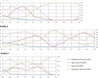
Landscape profile graphs effectively show the main charac-teristics of the urban–rural gradient using a 2-D space that allow the simultaneous analysis of the four above-mentioned indices (Fig. 13). In all graphs, the x-axis represents the dis-tance from the starting point of the profile; the left y-axis shows a percentage scale used for representing SDI and A-PLAND and N-A-PLAND curves; the right y-axis shows a probability scale used for representing SIDI curve.
In all the cases, the profile graphs indicate a similar land-scape composition and configuration at the very initial part of the three profiles. In this particular context, the small extents of high urbanised areas determine a particular initial compo-sition of the gradient that is not completely urban, since it is also characterised by agricultural and natural areas. Moving from the most urbanised area (the historical town centre) to-wards rural areas, SDI curves show a decreasing tendency, as expected, while A-PLAND and N-PLAND curves assume a different shape, indicating different types of urban-rural gra-dients in the three directions under investigation.
0.0 0.1 0.2 0.3 0.4 0.5 0.6 0.7
0 20 40 60 80 100
0.0 0.5 1.0 1.5 2.0 2.5 3.0 3.5 4.0 4.5 5.0
Profile 1
0.0 0.1 0.2 0.3 0.4 0.5 0.6 0.7
0 20 40 60 80 100
0.0 0.5 1.0 1.5 2.0 2.5 3.0 3.5 4.0 4.5 5.0 5.5 6.0
Profile 2
0.0 0.2 0.4 0.6 0.8
0 20 40 60 80 100
0.0 0.5 1.0 1.5 2.0 2.5 3.0 3.5
Profile 3
Settlement Density Index Agricultural PLAND Natural PLAND Simpson's Diversity Index
Fig. 13. Composition and diversity of the urban–rural gradient measured along the landscape profiles (year 2006). Settlement Density Index,
agricultural and natural percentages of landscape (PLAND), and Simpson’s Diversity Index (SIDI). The latter is represented using the right graduation on the graphs.
diversity and fragmentation. Along the other part of the pro-file, the two A-PLAND and N-PLAND curves assume a particular alternating behaviour, indicating the relative inci-dence of agricultural and natural areas and the position of the agricultural-forestry transitional areas, where SIDI increases as expected. The third profile illustrates another particular urban to rural gradient, with an initial steeper transition from the most urban to a natural-dominated agricultural landscape characterised by high values of diversity. The other section of the profile appears occupied by natural areas.
The transformations of the urban–rural gradient were stud-ied by means of a diachronic analysis of the four indices along the same landscape profiles (Fig. 14) and for all the time intervals defined. All the graphs indicate the variation of each index (positive or negative) occurred along the pro-file in a specific interval. SDI evolution was analysed on sep-arate graphs taking into account the different magnitude of the temporal variations of this index, while A-PLAND, N-PLAND and SIDI variations were plotted, for each profile, using three different graphs corresponding to the three peri-ods under investigation. This approach allowed an efficient spatio-temporal comparative analysis of the transformations of the urban–rural gradient composition and configuration in the study area.
As described above, the most relevant transformations of the landscape gradient took place in the 1955–1983 period.
S e tt le m ts D e n si ty In d e x 0 2 4 6 8
0.0 0.5 1.0 1.5 2.0 2.5 3.0 3.5 4.0 4.5 5.0
-0.5 -0.3 -0.1 0.1 0.3 0.5 -100 -50 0 50 100
0.0 0.5 1.0 1.5 2.0 2.5 3.0 3.5 4.0 4.5 5.0
-0.5 -0.3 -0.1 0.1 0.3 0.5 -100 -50 0 50 100
0.0 0.5 1.0 1.5 2.0 2.5 3.0 3.5 4.0 4.5 5.0
-0.5 -0.3 -0.1 0.1 0.3 0.5 -100 -50 0 50 100
0.0 0.5 1.0 1.5 2.0 2.5 3.0 3.5 4.0 4.5 5.0 0 2 4 6 8
0.0 0.5 1.0 1.5 2.0 2.5 3.0 3.5 4.0 4.5 5.0 5.5 6.0
-0.5 -0.3 -0.1 0.1 0.3 0.5 -100 -50 0 50 100
0.0 0.5 1.0 1.5 2.0 2.5 3.0 3.5 4.0 4.5 5.0 5.5 6.0
-0.5 -0.3 -0.1 0.1 0.3 0.5 -100 -50 0 50 100
0.0 0.5 1.0 1.5 2.0 2.5 3.0 3.5 4.0 4.5 5.0 5.5 6.0
-0.5 -0.3 -0.1 0.1 0.3 0.5 -100 -50 0 50 100
0.0 0.5 1.0 1.5 2.0 2.5 3.0 3.5 4.0 4.5 5.0 5.5 6.0 0 2 4 6 8
0.0 0.5 1.0 1.5 2.0 2.5 3.0 3.5
-0.5 -0.3 -0.1 0.1 0.3 0.5 -100 -50 0 50 100
0.0 0.5 1.0 1.5 2.0 2.5 3.0 3.5
-0.5 -0.3 -0.1 0.1 0.3 0.5 -100 -50 0 50 100
0.0 0.5 1.0 1.5 2.0 2.5 3.0 3.5
-0.5 -0.3 -0.1 0.1 0.3 0.5 -100 -50 0 50 100
0.0 0.5 1.0 1.5 2.0 2.5 3.0 3.5
Agricultural PLAND Natural PLAND Simpson's Diversity Index
1 9 5 5 -1 9 8 3 1 9 8 3 -1 9 9 4 1 9 9 4 -2 0 0 6
Profile 1 Profile 2 Profile 3
0
0 0 0 51955-1983 1 0 1 51983-19942 0 2 5 1994-20063 0 3 5
Fig. 14. Transformations of the urban–rural gradient measured along the landscape profiles (kilometres are shown on the x-axis). Spatial and
temporal variations of Settlement Density Index (SDI), of agricultural and natural percentages of landscape (A-PLAND and N-PLAND) and of Simpson’s Diversity Index (SIDI). The latter is represented using the right graduation on the graphs.
these modifications generated only small changes in land-scape configuration, also due to the efficacy of the GMP as outlined in Sect. 3.2.
4 Conclusions
The research is part of a wider study and is aimed at quan-tifying and interpreting LULC changes, particularly signifi-cant areas of the Mediterranean landscape. Similar to the re-sults of previous research carried out in other Italian Mediter-ranean landscapes (Fichera et al., 2012), in the last sixty years, the urbanisation process has considerably modified the landscape of Serra San Bruno municipality, with significant land-use conversions. This study has highlighted how un-derstanding the evolution of landscape trends, particularly where the urban/rural dynamic relations play a significant role, is crucial to their sustainable planning. As argued by Botequilla Leit˜ao et al. (2006), developing a basic under-standing of landscape changes is fundamental to weigh op-tions and consequences associated with alternative planning options, besides being the best way to deal with them. To that end, in a first phase, the integration of spatial, histori-cal (aerial photographs) and recent (orthophotos) data with
socio-economic data, in a geodatabase at a detailed scale, proved to be of great importance to understand the rela-tions between land-use, -cover and -funcrela-tions (Verburg et al., 2009). The observation and temporal analysis of LULC changes is a procedure that allows to identify ongoing trends and to better understand landscape evolution. Therefore, it is fundamental to implement tools helping to envisage fu-ture scenarios (Cerreta and De Toro, 2012; De Montis and Caschili, 2012; Fusco Girard and Torre, 2012). Furthermore, the analysis of LULC changes allows the temporal verifica-tion of the positive (e.g. reforestaverifica-tion of agricultural areas, land consolidation, etc.) or negative (lack of landscape plan-ning tools, agricultural abandonment, etc.) effects of past ter-ritorial policies. Finally, these analyses can allow the imple-mentation of landscape management tools and sustainable medium- and long-term landscape planning so as to direct future changes towards those which had positive effects and to contrast the past actions which had negative consequences on the landscape. This would have significant impacts not only at a local scale, which was the scope of this research, but also on regional-scale plans and programmes.
(Cerreta and De Toro, 2010; Cerreta et al., 2012; Cerreta and Mele, 2012), by providing helpful tools to spatially anal-yse and study landscape patterns, spatial variations and their most significant correlations.
Landscape profiling techniques for the analysis of the urban–rural gradient is an innovative and valuable approach for studying gradient characteristics over space and time. The landscape profile graphs allow a very effective diachronic analysis of the urban–rural gradient composition and config-uration. The strength of the approach is in its relative sim-ple applicability on every landscape context at the different scales of analysis and in the possibility to effectively com-pare more graphs referred to different areas under investi-gation. Certainly, the method needs further improvements, particularly in the selection of relevant metrics for better ex-ploration and analysis of landscape configuration. Moreover, additional research is needed for deeper comprehension of the relations between graph shapes and landscape functions. Future developments of this research will include the use of WorldView-2 imagery in order to compare automatic land cover classification using object-oriented analysis and auto-matic settlement extraction comparing different data sources.
Acknowledgements. The authors would like to thank DigitalGlobe® for providing the Worldview-2 imagery under the Erdas Imagine-DigitalGlobe 2012 Geospatial Challenge Contest.
Edited by: H. Asche
References
Aguilera, F., Valenzuela, L. M., and Botequilha-Leit˜ao, A.: Land-scape metrics in the analysis of urban land use patterns: A case study in a Spanish metropolitan area, Landscape Urban Plan., 99, 226–238, doi:10.1016/j.landurbplan.2010.10.004, 2011. Alberti, M., Solera, G., and Tsetsi, V.: La citt`a sostenibile
(Sustain-able Cities), Franco Angeli, Milano, Italy, 1994.
Antrop, M.: Changing patterns in the urbanized country-side of Western Europe, Landscape Ecol., 15, 257–270, doi:10.1023/A:1008151109252, 2000.
Antrop, M.: Landscape change and the urbanization pro-cess in Europe, Landscape and Urban Plan, 67(1-4), 9–26, doi:10.1016/S0169-2046(03)00026-4, 2004.
Bhatta, B.: Analysis of urban growth pattern using remote sensing and GIS: A case study of Kolkata, India, Int. J. Remote Sens., 30, 4733–4746, doi:10.1080/01431160802651967, 2009.
Blasi, C., Capotorti, G., Smiraglia, D., Guida, D., Zavattero, Z., Mollo, B., Frondoni, R., and Copiz, R.: The Ecoregions of Italy, A thematic contribution to the National Biodiversity Strategy, available at: www.minambiente.it/export/sites/default/archivio/ biblioteca/protezione natura/ecoregioni italia eng.pdf (last ac-cess: 20 September 2012), 2010.
Blondel, J.: The “Design” of Mediterranean Landscapes: A Millen-nial Story of Humans and Ecological Systems during the His-toric Period, Hum. Ecol., 34, 713–729, doi:10.1007/s10745-006-9030-4, 2006.
B¨ohner, J., McCloy, K. R., and Strobl, J. (Eds.): SAGA – Analysis and Modelling Applications, G¨ottinger Geographische Abhand-lungen, Germany, Vol. 115, 130 pp, 2006.
Botequilha Leit˜ao, A., Miller, J., Ahern, J., and McGarigal, K.: Measuring landscapes: A planner’s handbook, Island Press, Washington DC, USA, 2006.
Botequilha Leit˜ao, A. and Ahern, J.: Applying landscape eco-logical concepts and metrics in sustainable landscape plan-ning, Landscape Urban Plan., 59, 65–93, doi:10.1016/S0169-2046(02)00005-1, 2002.
Braimoh, A. K.: Random and systematic land-cover transitions in northern Ghana, Agriculture, Ecosyst. Environ., 113, 254–263, doi:10.1016/j.agee.2005.10.019, 2006.
Cerreta, M. and De Toro, P.: Integrated spatial assessment for a creative decision-making process: a combined methodological approach to strategic environmental assessment, Int. J. Sustain. Dev., 13, 17–30, doi:10.1504/IJSD.2010.035096, 2010. Cerreta, M. and De Toro, P.: Assessing urban transformations:
a SDSS for the master plan of Castel Capuano, Naples, ICCSA 2012, Part II, Lect. Notes Comput. Sc., 7334/2012, 168– 180, doi:10.1007/978-3-642-31075-1 13, 2012.
Cerreta, M. and Mele, R.: A landscape complex values map: inte-gration among soft values and hard values in a spatial decision support system, ICCSA 2012, Part II, Lect. Notes Comput. Sc., 7334/2012, 653–669, doi:10.1007/978-3-642-31075-1 49, 2012. Cerreta, M., Panaro, S., and Cannatella, D.: Multidimensional spatial decision-making process: local shared values in action, ICCSA 2012, Part II, Lect. Notes Comput. Sc., 7334/2012, 54– 70, doi:10.1007/978-3-642-31075-1 5, 2012.
Cihlar, J.: Land cover mapping of large areas from satellites: Sta-tus and research priorities, Int. J. Remote Sens., 21, 1093–1114, doi:10.1080/014311600210092, 2000.
Cushman, S. A., McGarigal, K., and Neel, M. C.: Parsimony in landscape metrics: Strength, universality, and consistency, Ecol. Indic., 8, 691–703, doi:10.1016/j.ecolind.2007.12.002, 2008. Danese, M., Lazzari, M., and Murgante, B.: Kernel density
estima-tion methods for a geostatistical approach in seismic risk anal-ysis: The case study of Potenza hilltop town (southern Italy), ICCSA 2008, Part I, Lect. Notes Comput. Sc., 5072/2008, 415– 429, doi:10.1007/978-3-540-69839-5 31, 2008.
De Montis, A. and Caschili, S.: Nuraghes and land-scape planning: Coupling viewshed with complex net-work analysis, Landscape Urban Plan., 105, 315–324, doi:10.1016/j.landurbplan.2012.01.005, 2012.
Defries, R. S., Foley, J. A., and Asner, G. P.: Land-use choices: balancing human needs and ecosystem func-tion, Front Ecol. Environ., 2, 249–257, doi:10.1890/1540-9295(2004)002[0249:LCBHNA]2.0.CO;2, 2004.
Di Fazio, S., Modica, G., and Zoccali, P.: Evolution Trends of Land Use/Land Cover in a Mediterranean Forest Landscape in Italy, ICCSA 2011, Part I, Lect. Notes Comput. Sc., 6782/2011, 284– 299, doi:10.1007/978-3-642-21928-3 20, 2011.
EEA – European Environment Agency: European forest types, EEA Technical report no. 9, available at: www.eea.europa.eu/ publications/technical report 2006 9 (last access: 18 Septem-ber 2012), 2006a.
EEA – European Environment Agency: Urban sprawl in Europe: The ignored challenge, EEA Report no. 10/2006, Publications Office of the European Union, Luxembourg, 2006b.
EEA – European Environment Agency: Landscape fragmentation in Europe, Joint EEA-FOEN report no. 2/2011, EEA Report se-ries, Publications Office of the European Union, Luxembourg, doi:10.2800/78322, 2011.
Farina, A.: Principles and methods in landscape ecology, Chap-man & Hall, London, UK, 1998.
Fichera, C. R., Modica, G., and Pollino, M.: GIS and Remote Sensing to Study Urban-Rural Transformation During a Fifty-Year Period, ICCSA 2011, Part I, Lect. Notes Comput. Sc., 6782/2011, 237–252, doi:10.1007/978-3-642-21928-3 17, 2011. Fichera, C. R., Modica, G., and Pollino, M.: Land Cover classifica-tion and change-detecclassifica-tion analysis using multi-temporal remote sensed imagery and landscape metrics, Eur. J. Remote Sens., 45, 1–18, doi:10.5721/EuJRS20124501, 2012.
Foley, J. A., Defries, R., Asner, G. P., Barford, C., Bonan, G., Car-penter, S. R., Chapin, F. S., Coe, M. T., Daily, G. C., Gibbs, H. K., Helkowski, J. H., Holloway, T., Howard, E. A., Kucharik, C. J., Monfreda, C., Patz, J. A., Prentice, I. C., Ramankutty, N., and Snyder, P. K.: Global consequences of land use, Science, 309, 570–574, doi:10.1126/science.1111772, 2005.
Forman, R. T. T.: Land Mosaics: The Ecology of Landscapes and Regions, Cambridge University Press, Cambridge, UK, 1995. Fusco Girard, L. and De Toro, P.: Integrated spatial assessment: a
multicriteria approach to sustainable development of cultural and environmental heritage in San Marco dei Cavoti, Italy, Centr. Eur. J. Operat. Res., 15, 281–299, doi:10.1007/s10100-007-0031-1, 2007.
Fusco Girard, L. and Torre, C.: The use of ahp in a multiac-tor evaluation for urban development programs: a case study, ICCSA 2012, Part II, Lect. Notes Comput. Sc., 7334/2012, 157– 167, doi:10.1007/978-3-642-31075-1 12, 2012.
Gatrell, A. C., Bailey, T. C., Diggle, P. J., and Rowlingson, B. S.: Spatial Point Pattern Analysis and Its Application in Geo-graphical Epidemiology, T. Inst. British Geogr., 21, 256–274, doi:10.2307/622936, 1996.
Gomarasca, M.: Basics of Geomatics, Springer, the Netherlands, doi:10.1007/978-1-4020-9014-1, 2009.
Gustafson, E. J.: Minireview: Quantifying Landscape Spatial Pat-tern: What Is the State of the Art?, Ecosystems, 1, 143–156, doi:10.1007/s100219900011, 1998.
Hahs, A. K. and McDonnell, M. J.: Selecting independent measures to quantify Melbourne’s urban–rural gradient, Landscape Ur-ban Plan., 78, 435–448, doi:10.1016/j.landurbplan.2005.12.005, 2006.
Hasse, J. E. and Lathrop, R. G.: Land resource impact indicators of urban sprawl, Appl. Geogr., 23, 159–175, doi:10.1016/j.apgeog.2003.08.002, 2003.
Herold, M., Goldstein, N. C., and Clarke, K. C.: The spatiotem-poral form of urban growth: measurement, analysis and model-ing, Remote Sens. Environ., 86, 286–302, doi:10.1016/S0034-4257(03)00075-0, 2003.
Herold, M., Couclelis, H., and Clarke, K.: The role of spatial metrics in the analysis and modeling of urban land use change, Comput. Environ. Urban, 29, 369–399, doi:10.1016/j.compenvurbsys.2003.12.001, 2005.
Hidding, M., Needham, B., and Wisserhof, J.: Discourses of town and country, Landscape Urban Plan., 48, 121–130, doi:10.1016/S0169-2046(00)00036-0, 2000.
Hoffhine Wilson, E., Hurd, J. D., Civco, D. L., Prisloe, M. P., and Arnold, C.: Development of a geospatial model to quantify, de-scribe and map urban growth, Remote Sens. Environ., 86, 275– 285, doi:10.1016/S0034-4257(03)00074-9, 2003.
Jones, M. C., Marron, J. S., and Sheather, S. J.: A Brief Survey of Bandwidth Selection for Density Estimation, J. Am. Stat. Assoc., 91, 401–407, 1996.
Kong, F. and Nakagoshi, N.: Spatial-temporal gradient analysis of urban green spaces in Jinan, China, Landscape Urban Plan., 78, 147–164, doi:10.1016/j.landurbplan.2005.07.006, 2006. Kong, F., Yin, H., Nakagoshi, N., and James, P.:
Simu-lating urban growth processes incorporating a poten-tial model with spapoten-tial metrics, Ecol. Indic., 20, 82–91, doi:10.1016/j.ecolind.2012.02.003, 2012.
Li, H. and Wu, J.: Use and misuse of
land-scape indices, Landscape Ecol., 19, 389–399,
doi:10.1023/B:LAND.0000030441.15628.d6, 2004.
Lillesand, T., Kiefer, R., and Chipman, J.: Remote sensing and im-age interpretation, 5th Edn., Wiley, New York, 2003.
Lloyd, C. D.: Local models for spatial analysis. CRC Press Taylor & Francis Group, Boca Raton, FL, doi:10.1201/EBK1439829196, 2007.
Lu, D., Mausel, P., Brondizio, E., Moran, E., and Brond´ızio, E.: Change detection techniques, Int. J. Remote Sens., 25, 2365– 2401, doi:10.1080/0143116031000139863, 2004.
Luck, M. and Wu, J.: A gradient analysis of urban land-scape pattern: a case study from the Phoenix metropoli-tan region, Arizona, USA, Landscape Ecol., 17, 327–339, doi:10.1023/A:1020512723753, 2002.
McDonnell, M. J. and Hahs, A. K.: The use of gradient analysis studies in advancing our understanding of the ecology of urban-izing landscapes: current status and future directions, Landscape Ecol., 23, 1143–1155, doi:10.1007/s10980-008-9253-4, 2008. McDonnell, M. J. and Pickett, S. T. A.: Ecosystem Structure and
Function along Urban-Rural Gradients: An Unexploited Oppor-tunity for Ecology, Ecology, 71, 1232, doi:10.2307/1938259, 1990.
McGarigal, K. and Cushman, S. A.: The gradient concept of land-scape structure, in: Issues and Perspectives in Landland-scape Ecol-ogy, edited by: Wiens, J. and Moss, M., Cambridge University Press, Cambridge, UK, 112–119, 2005.
Mercurio, R.: Restauro della foresta mediterranea (Restoration of the Mediterranean Forest), Clueb, Bologna, Italy, 368 pp., 2010. Murgante, B. and Danese, M.: Urban versus Rural: the decrease of agricultural areas and the development of urban zones analyzed with spatial statistics, Int. J. Agr. Environ. Inform. Syst., 2, 16– 28, doi:10.4018/jaeis.2011070102, 2011.
Myers, N., Mittermeier, R., and Mittermeier, C.: Biodiversity hotspots for conservation priorities, Nature, 403, 853–858, doi:10.1038/35002501, 2000.
Nagendra, H.: Opposite trends in response for the Shannon and Simpson indices of landscape diversity, Appl. Geogr., 22, 175– 186, doi:10.1016/S0143-6228(02)00002-4, 2002.
Neri, M., Menconi, M. E., Vizzari, M., and Mennella, V.: A proposal of a new methodology for best location of environ-mentally sustainable roads infrastructures. Validation along the Fabriano-Muccia road, Informes de la Construcci´on, 517, 101– 112, doi:10.3989/ic.09.043, 2010.
Ode, A., Tveit, M. S., and Fry, G.: Advantages of using˚ different data sources in assessment of landscape change and its effect on visual scale, Ecol. Indic., 10, 24–31, doi:10.1016/j.ecolind.2009.02.013, 2010.
Peng, J., Wang, Y., Zhang, Y., Wu, J., Li, W., and Li, Y.: Evaluating the effectiveness of landscape metrics in quantifying spatial patterns, Ecol. Indic., 10, 217–223, doi:10.1016/j.ecolind.2009.04.017, 2010.
Perchinunno, P., Rotondo, F., and Torre, C.: The Evidence of Links between Landscape and Economy in a Rural Park, Int. J. Agr. Environ. Inform. Syst., 3, 1–14, doi:10.4018/jaeis.2012070105, 2012.
Perella, G., Galli, A., and Marcheggiani, E.: The Potential of Ecomuseums in Strategies for Local Sustainable De-velopment in Rural Areas, Landscape Res., 35, 431–447, doi:10.1080/01426397.2010.486854, 2010.
Poelmans, L. and Van Rompaey, A.: Detecting and modelling spa-tial patterns of urban sprawl in highly fragmented areas: A case study in the Flanders–Brussels region, Landscape Urban Plan., 93, 10–19, doi:10.1016/j.landurbplan.2009.05.018, 2009. Quezel, P. and Medail, F.: Ecologie et biog´eographie des forets du
bassin m´editerran´een, Elsevier, Paris, 576 pp., 2003.
Selicato, M., Torre, C., and Trofa, G. L.: Prospect of integrate monitoring: a multidimensional approach, ICCSA 2012, Part II, Lect. Notes Comput. Sc., 7334/2015, 144–156, doi:10.1007/978-3-642-31075-1 11, 2012.
Seto, K. C. and Fragkias, M.: Quantifying Spatiotemporal Pat-terns of Urban Land-use Change in Four Cities of China with Time Series Landscape Metrics, Landscape Ecol., 20, 871–888, doi:10.1007/s10980-005-5238-8, 2005.
Shannon, C. E. and Weaver, W.: The mathematical theory of com-munication, University of Illinois Press, Urbana, IL, 1949. Silverman, B. W., Jones, M. C., Fix, E., and Hodges, J. L.: An
Important Contribution to Nonparametric Discriminant Analysis and Density Estimation: Commentary on Fix and Hodges (1951), Int. Stat. Rev., 57, 233–247, doi:10.2307/1403796, 1989.
Simpson, E. H.: Measurement of diversity, Nature, 163, p. 688, doi:10.1038/163688a0, 1949.
Smith, M. J., Goodchild, M. F., and Longley, P. A.: Geospatial Analysis: A Comprehensive Guide to Principles, Techniques and Software Tools, Troubador Publishing, Leicester, UK, 2007. Sudhira, H. S., Ramachandra, T. V., and Jagadish, K. S.: Urban
sprawl: metrics, dynamics and modelling using GIS, Int. J. Appl. Earth Obs., 5, 29–39, doi:10.1016/j.jag.2003.08.002, 2004. Torrens, P. A. and Alberti, M.: Measuring sprawl, CASA
Cen-tre for Advanced Spatial Analysis, Working paper 27, avail-able at: www.bartlett.ucl.ac.uk/casa/pdf/paper27.pdf, last access: 24 July 2012, University College London, London, 2000. Turner, M. G. and Ruscher, C. L.: Changes in landscape
patterns in Georgia, USA, Landscape Ecol., 1, 241–251, doi:10.1007/BF00157696, 1988.
Updike, T. and Comp, C.: Radiometric use of WorldView-2 im-agery, Technical Note, DigitalGlobe Inc., 2010.
Uuemaa, E., Antrop, M., Roosaare, J., Marja, R., and Mander, ¨
U.: Landscape Metrics and Indices: An Overview of Their Use in Landscape Research, Living Rev. Landscape Res., 3, 1– 28, available at: www.livingreviews.org/lrlr-2009-1 (last access: 25 July 2012), 2009.
Verburg, P. H., Koning, G. H. J., Kok, K., Veldkamp, A., and Priess, J.: The CLUE modelling framework: an integrated model for the analysis of land use change, in: Land Use and Cover Change, edited by: Singh, R. B., Jefferson, F., and Himiyama, Y., Science Publishers, Enfield, NH, 11–25, 2001.
Verburg, P. H., van de Steeg, J., Veldkamp, A., and Willemen, L.: From land cover change to land function dynamics: a major chal-lenge to improve land characterization, J. Environ. Manage., 90, 1327–1335, doi:10.1016/j.jenvman.2008.08.005, 2009. Vitousek, P. M.: Human Domination of Earth’s Ecosystems,
Sci-ence, 277, 494–499, doi:10.1126/science.277.5325.494, 1997. Vizzari, M.: Spatio-temporal analysis using urban-rural gradient
modelling and landscape metrics, ICCSA 2011, Part I, Lect Notes Comput Sc, 6782/2011, 103–118, doi:10.1007/978-3-642-21928-3 8, 2011a.
Vizzari, M.: Spatial modelling of potential landscape quality, Appl. Geogr., 31, 108–118, doi:10.1016/j.apgeog.2010.03.001, 2011b. Weng, Y. C.: Spatiotemporal changes of landscape pattern in re-sponse to urbanization, Landscape Urban Plan., 81, 341–353, doi:10.1016/j.landurbplan.2007.01.009, 2007.
Wu, J. and Hobbs, R.: Key issues and research priorities in land-scape ecology: an idiosyncratic synthesis, Landland-scape Ecol., 17, 355–365, doi:10.1023/A:1020561630963, 2002.
Yang, Y., Zhou, Q., Gong, J., and Wang, Y.: Gradient analy-sis of landscape spatial and temporal pattern changes in Bei-jing metropolitan area, Sci. China Technol. Sci., 53, 91–98, doi:10.1007/s11431-010-3206-2, 2010.