https://doi.org/10.5194/amt-10-4761-2017 © Author(s) 2017. This work is distributed under the Creative Commons Attribution 3.0 License.
Correcting negatively biased refractivity below ducts in GNSS radio
occultation: an optimal estimation approach towards improving
planetary boundary layer (PBL) characterization
Kuo-Nung Wang1, Manuel de la Torre Juárez1, Chi O. Ao1, and Feiqin Xie2
1Jet Propulsion Laboratory, California Institute of Technology, 4800 Oak Grove Drive, Pasadena, CA 91109, USA 2Texas A & M University – Corpus Christi, 6300 Ocean Dr., Corpus Christi, TX 78412, USA
Correspondence to:Kuo-Nung Wang ([email protected]) Received: 10 April 2017 – Discussion started: 21 April 2017
Revised: 26 August 2017 – Accepted: 9 October 2017 – Published: 8 December 2017
Abstract. Global Navigation Satellite System (GNSS) ra-dio occultation (RO) measurements are promising in sens-ing the vertical structure of the Earth’s planetary boundary layer (PBL). However, large refractivity changes near the top of PBL can cause ducting and lead to a negative bias in the retrieved refractivity within the PBL (below ∼2 km). To remove the bias, a reconstruction method with assump-tion of linear structure inside the ducting layer models has been proposed by Xie et al. (2006). While the negative bias can be reduced drastically as demonstrated in the simula-tion, the lack of high-quality surface refractivity constraint makes its application to real RO data difficult. In this paper, we use the widely available precipitable water (PW) satel-lite observation as the external constraint for the bias cor-rection. A new framework is proposed to incorporate opti-mization into the RO reconstruction retrievals in the pres-ence of ducting conditions. The new method uses optimal estimation to select the best refractivity solution whose PW and PBL height best match the externally retrieved PW and the known a priori states, respectively. The near-coincident PW retrievals from AMSR-E microwave radiometer instru-ments are used as an external observational constraint. This new reconstruction method is tested on both the simulated GNSS-RO profiles and the actual GNSS-RO data. Our re-sults show that the proposed method can greatly reduce the negative refractivity bias when compared to the traditional Abel inversion.
1 Introduction
The planetary boundary layer (PBL) is the lowest layer of the atmosphere (∼2 km) and couples the surface to the free troposphere. Influenced mainly by surface friction, solar ra-diation, and turbulent transport of moisture, the PBL con-trols the energy distribution from the surface into the at-mosphere. Through the turbulent winds along with cumuli-form and straticumuli-form clouds cumuli-formation, the PBL can greatly affect the local weather as well as the global climate (Gar-ratt, 1992). Due to its importance to the weather prediction community, the PBL has been extensively studied with vari-ous sounding techniques for several decades.
RO over other passive remote sensing instruments (Curran, 1989). Additionally, the L-band GNSS RO signals can pene-trate through clouds and precipitation (Solheim et al., 1999), which are common at the height at the top of the PBL. These features make GNSS RO a valuable tool for sensing the PBL (Guo et al., 2011; Ao et al., 2012; Xie et al., 2012; Chan and Wood, 2013; Ho et al., 2015).
However, it is known that the large refractivity change as-sociated with a strong inversion layer at the top of the PBL can cause severe negative biases in RO refractivity measure-ments (N-bias) (Sokolovskiy, 2003; Xie et al., 2006; Ao, 2007). The large temperature and moisture changes near the top of the PBL could lead to a sharp negative refractiv-ity gradient such that the radius of curvature of the signal path can become less than the radius of the Earth. This phe-nomenon, called ducting, occurs when the refractivity gra-dient dN/dr.−157 (N-units km−1) and can be frequently observed in the subtropics below 2 km. The layer where the ducting occurred is called the ducting layer. Due to the trans-mitter and receiver geometry of GNSS RO, the tangent point of each ray path is never located within the ducting lay-ers, which theoretically can “trap” the signal whose tangent point is inside. As a result, the GNSS-RO bending angle mea-surements will lose the information inside the ducting layer, in which the information cannot be recovered using solely GNSS-RO observations. The standard Abel inversion of the bending angle profile will always lead to a profile with no ducts and can cause a negative N-bias as large as 15 % be-low the ducting layer (Xie et al., 2010). Correcting the N -bias within the PBL is essential towards the use of RO in studying the vertical structure within the PBL. While the weather analyses can assimilate RO bending angles, which are unaffected by the refractivity bias caused by ducting, it is not clear that the analyses can optimally handle these high-vertical-resolution measurements. In addition, the analyses may be strongly affected by bias in the model, as evidenced by the low PBL height over the stratocumulus regions (Xie et al., 2012). Therefore, it is of great scientific interests to retrieve an unbiased PBL refractivity based on observations only.
To mitigate theN-bias and reconstruct refractivity profiles inside the boundary layer, a reconstruction method was pro-posed by Xie et al. (2006), hereinafter referred to as (Xie06). The paper confirmed that an infinite number of refractivity profiles correspond to one bending angle profile in the pres-ence of ducting conditions. A nonlinear function used to de-scribe the continuum of refractivity solutions was derived based on the Abel-retrieved refractivity profile. Choosing the correct parameter and profile from the continuum, however, depends on two assumptions that cannot be easily fulfilled. First, to use the surface refractivity constraint, the RO bend-ing angle measurements are implicitly assumed to cover all altitudes and stop exactly at the Earth’s surface. However, the real RO bending angle profiles often do not reach the surface due to a combination of receiver measurement errors and
at-mospheric variabilities (Ao et al., 2012). Second, the recon-struction method assumes that the top height of the ducting layer can be determined accurately. However, due to the high variability in the bending angle, identifying the impact pa-rameter of the ducting layer in the real occultation could be challenging.
In this paper we present a new and improved reconstruc-tion method that implements optimal estimareconstruc-tion along with external measurements of precipitable water (PW) based on a modification of the Xie06 approach. In Sect. 2, the ducting effects and the reconstruction method in Xie06 are reviewed and our new approach using optimal estimation is described. The results for radiosonde observation (RAOB) using the op-timal estimation approach and the comparison with different PW observation sources are presented in Sect. 3. In Sect. 4 we validate actual GNSS-RO data results using the proposed reconstruction method. The summaries and conclusions are provided in Sect. 5.
2 Refractivity reconstruction method 2.1 N-bias
Under the assumption of a spherically symmetric atmo-sphere, the impact parametera of a single ray path can be defined as
a=rn (r)sinφ, (1)
wheren is the refractive index, r is the distance from the center of curvature to each point of the ray path, andφis the angle between the ray path and the radial vector. The accu-mulated bending angle of a GNSS-RO ray path can be calcu-lated for a refractivity profile as (Fjeldbo et al., 1971)
α (rt)= −2n (rt) rt ∞ Z rt 1 n (r) dn (r) dr dr p
[n (r) r]2−[n (r t) rt]2
, (2)
where α is the bending angle and rt is the radius of the ray path at the tangent point. To retrieve the refractivity information from the bending angle measurement, Eq. (2) can be simplified by using the impact parameter defined as a=n (rt) rt(φ=90◦in Eq. (1) at the tangent point) and as-suming that the functionx=n (r) ris monotonically increas-ing withr:
α (a)= −2a ∞ Z a 1 n dn dx dx √
x2−a2 (3)
so that the refractive index can be derived analytically as (Fjeldbo et al., 1971)
n (x)=exp 1 π ∞ Z x
α (a)da
√
a2−x2
which is called the Abel-inversion integral.
The Abel inversion is extensively used in RO retrievals, based on the fact that in most cases the one-to-one relation-ship between the derived refractivity profile and the mea-sured bending angle profile is valid. However, this relation-ship breaks down when ducting occurs (Sokolovskiy, 2003). 2.1.1 Ducting effects
The refractivity in the neutral atmosphere is related to atmo-spheric temperature, pressure, and the water vapor pressure with the following equation (Smith and Weintraub, 1953): N =77.6p
T +3.73×10 5 e
T2, (5)
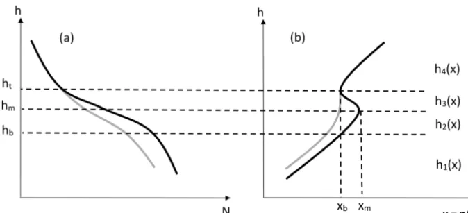
whereN=(n−1)×106is the refractivity inN-units,nis the refractive index, pis pressure in millibar,T is temperature in degrees Kelvin, and eis the water vapor pressure in mil-libar. Due to the large change in temperature and moisture, the refractivity decreases rapidly across the top of the PBL as seen in Fig. 1a between the heighthm andht. The duct-ing condition occurs when the refractivity gradient exceeds the critical refraction; i.e., dN/dr.−157 (N-units km−1), wherex (r)=n (r) r is no longer a monotonic function with respect tor. The heighthis defined (Sokolovskiy, 2003) as
h=r−re, (6)
wherereis the radius of curvature at the Earth’s surface. As illustrated in Fig. 1b, the functionh(x), shown in black, can be divided into four intervals:h1(x), wherexincreases from the surface to the heighthbto reachxb;h2(x), wherex fur-ther increases toxm, fromhbtohm;h3(x), which is the duct-ing layer with refractivity gradient exceedduct-ing critical refrac-tion, wherex decreases fromxmathmback toxbatht; and h4(x), wherex increases again fromht and the monotonic relation betweenx andris restored. Within the intervals of h2(x)andh3(x), the changing signs of the slopes result in a non-monotonic relationship betweenhandx.
For simplicity, here, we define the trapping layer, which includes the ducting layer and the layer underneath fromhb to ht where the monotonic characteristic of h(x)vanishes. Inside the trapping layer, the refractivity gradient is large enough to trap the signal with a tangent point betweenhband htand cause an infinite bending angle in its ray path. Because of the geometry of GNSS RO, in which both the transmitter and the receiver are located outside the Earth’s atmosphere, the tangent points of the received signals do not appear inside the trapping layer. In other words, the information between hbandht is lost in the received signal, and the bending an-gle observation is not able to cover this gap. This gap can be noticed by examining Eq. (2). When evaluating the bending angle with Eq. (2) inside the trapping layer,hb< rt−re< ht, the termn(r)rabove the heightrtbecomes less thann(rt)rt because of the negative gradient of x between hm and ht. This would lead to a negative value inside the square root
in Eq. (2) and the solution would be a complex number for the bending angle inside the trapping layer which is unphys-ical. However, all the bending angles belowhb can still be evaluated as the monotonic relationship ofh(x)is in place. Namely, the rays with tangent points below the trapping layer can still penetrate through the trapping layer and arrive at the receiver, and so the bending angle of these rays can still be calculated by GNSS RO.
Although the missing bending angle measurements in the trapping layer cause a gap in theα−rrelationship, theα−a relationship, will remain seamless because thexvalue at the top and the bottom of the trapping layer are identical (e.g.,xb in Fig. 1b). Therefore, we can still apply the standard Abel in-version upon the bending angle profile in the presence of the ducting. However, since thex(r)function is not monotonic within the trapping layer, the standard Abel inversion Eq. (4), which assumes monotonicx, will lead to erroneous refractiv-ity results belowht. While the refractivity retrieval remains valid aboveht, the bending contribution inside the trapping layer is missing from the standard Abel inversion belowxb. Consequently, the Abel-retrieved refractivity below xb will be negatively biased (negativeN bias) (Sokolovskiy, 2003; Xie et al., 2006; Ao, 2007) which are shown as the grey curves in Fig. 1a and b. To correct the GNSS-RO refractivity retrieval bias in the presence of the ducting layer inside the PBL, a bilinear trapping layer model along with a reconstruc-tion method were proposed by Xie06, which is described in the next subsection.
2.1.2 Bilinear trapping layer model and the reconstruction method
Xie06 demonstrated that an infinite number of refractivity so-lutions can generate the same bending angle observation us-ing Eq. (2). Among all the refractivity solutions correspond-ing to the same bendcorrespond-ing angle profile, the one retrieved by the standard Abel inversion introduces the largest negative bias. To mathematically describe each solution, Xie06 assume that theh(x)depicted in Fig. 1b can be approximated by a sim-ple bilinear model, e.g., two connected straight line segments inside the trapping layer betweenhbandht:
h2(x)=hb+
hm−hb xm−xb
(x−xb) , (7)
h3(x)=ht− ht−hm xm−xb
(x−xb) . (8)
Under this assumption, the missing information inside the trapping layer can be recovered by the parameterization of theh(x)betweenhbandht, and theh1(x)at segment 1 can be derived analytically for given parametersxb,xm,hb, and ht:
h1(x)=hA(x)+ 2
π(ht−hb) h
z−1+z2tan−1(1/z)i, (9) wherehA(x)is the height function with respect toxfrom the
Figure 1.The illustration of the corresponding refractivity profile(a)and theh(x)function(b)when ducting occurs. The true profiles are shown in black and the profiles acquired by GNSS-RO Abel retrievals are shown in grey. The large refractivity gradient betweenhmandht
causes the negative slope ofh3(x)and the multivalued functionh(x)betweenxbandxm.
z=√xb−x/
√
xm−xb. By using Eq. (9), all the possible re-fractivity profile solutions, or the continuum of the solutions, belowhtcan be produced given five parameters defining the trapping layer:xb,xm,hb,hm, andht.
To identify the best refractivity solution out of the contin-uum of the solutions, additional assumptions and constraints were proposed:
A1. The height of the trapping layer top (ht) is needed and can be derived from the standard Abel-retrieved refrac-tivity profile. Due to the large bending angle (theoreti-cally→ ∞) near both the top and bottom of the trap-ping layer, the peak in the bending angle profile is as-sumed to be detectable and its corresponding impact pa-rameter (xb) can be identified accurately. The height of the trapping layer topht, therefore, can be calculated in the Abel-inversion profile at the point with knownxb. However, accurate detection of the trapping layer top is challenging in practice as it relies on the high-resolution bending angle profile which could be very noisy with-out filtering. On the other hand, the filtering process re-duces the vertical resolution, which leads to error in the parameterxb. Therefore, a more robust method to detect xbparameter is needed.
A2. The standard Abel-retrieved refractivity profile near the top of the trapping layer behaves like a square-root function. Expanding by Taylor series aroundz=0, the Abel-inversion result functionhA(x)can be written as
hA(x)=ht− 4
π(ht−hb)z+(h3−h2)z 2
+O(z3). (10)
Keeping the leading order term in z, the function hA(x)−ht is assumed to behave like a parabola near
xband the derivative of its square can be written as d
dx[hA(x)−ht] 2|
x→x−b = −C (11)
so thatC can be determined through linear regression inhA(x) over 200 m belowxb (Xie et al., 2006). By neglecting higher-order terms of the derivative,C can be expressed as
C' 16
π2
(ht−hb)2 xm−xb
. (12)
Since the parametersxb andht are known, afterC is determined the parameterxmcan be calculated givenhb using Eq. (12).
A3. Based on global observations of high-vertical-resolution sounding over the ocean, the slope ofh1(x)is assumed to be continuous athb to the bottom of the trapping layer:
dh1(x) dx
x→x−b
= dh2(x)
dx
x→xb+
. (13)
This assumption determines the parameterhmby linear extrapolation ofh1(x)untilx=xm.
Up to this point, all five parameters are connected so that once the parameterhbis given the other four can be determined. However, while a large number ofhb val-ues can be used in a single GNSS-RO case to generate a family of candidate profiles, choosing the correct pro-file from the family is still challenging. To determine the hbparameter one needs an additional constraint. A4. The surface refractivity constraint is applied, which
re-quires the extension of the RO bending angle observa-tion to the Earth’s surface,x0,
i.e., from the whole family of refractivity profiles only the one with minimum height starting at zero will be chosen as the best solution of the reconstructed profile. However, for a number of reasons, including measure-ment noise and tracking error, horizontal variability, and diffraction effects, the retrieved profiles do not often reach the Earth’s surface (Ao et al., 2012). Thus, the surface constraint is very difficult to fulfill and becomes the main obstacle in applying the reconstruction method in practice.
As shown above, the reconstruction method in Xie06 de-pends upon several conditions which may not be achievable. In this paper, we aim to refine this reconstruction method by improving the applicability of (A1) and replacing the surface refractivity constraint in (A4) with the combination of opti-mal estimation along with the external PW observation con-straint. Furthermore, an improved method to determine the trapping layer top (xb) is proposed and the bilinear parame-terization model of the trapping layer is modified to reflect the smoother and more realistic structure of theh(x)curve. 2.2 Optimal estimation implementation
Our approach retains Eq. (9) from Xie06 as the core concept of the retrieval method. First, to improve the determination of the height of the ducting layer, a refined algorithm is de-veloped, which no longer determines xb only by the noisy bending angle profile but also through optimal estimation it-erations. Secondly, the retrieved PW from ancillary data is used to replace the surface constraint in (A4) (Xie06). This research focuses on correcting theN-bias below the trapping layer and deriving the key parameters such as duct altitude, thickness, and refractivity gradient information.
To implement these two major changes to the reconstruc-tion algorithm, the basic parameterizareconstruc-tion process needs to be modified as described in the following subsection. 2.2.1 Parameterization
In the Xie06 reconstruction method, all five parameters are connected and only one free parameter,hb, is needed to de-fine each refractivity profile. To relax the xb determination constraint in (A1), we use a different approach.
First, the highest 100 m of h1(x)will be replaced by the linear extrapolation from below; its slope is determined by linear regression between 100 and 200 m below the height hb. The reason is that the top of the analytical solution cal-culated by Eq. (9) is sensitive to the mis-modeling ofh2(x) and h3(x), which are assumed to be bilinear segments be-tweenhbandht. Spurious spikes and fluctuations are found at the top 100 m of the functionh1(x)if the straight line as-sumption inside the critical layer is violated by the data or the parameters, e.g.,hb, are not appropriately estimated from Equation (12). While these fluctuations inh1(x)are usually small (<20 m) and typically occur within 100 m belowhb,
they can significantly change the slope athb, which makes theh2(x)value obtained from assumption A3 inconsistent with having one refractivity for each impact parameter be-lowhb. Therefore, we replaced the top portion ofh1(x)with a linear extension of the curve below to remove the fluctua-tion. Note that the variablehbchanges when the top ofh1(x) is replaced. To avoid the inconsistency between the newhb and the originally specifiedhb,xm is chosen overhbas the “free” variable to construct a profile inside and below the critical layer.
Second, instead of assumingxbas known, both parameters xbandxmare used as “free” variables as ishbin the Xie06 approach. Namely, a pair ofxb andxm are required to de-termine one refractivity profile in this new parameterization model. With both modifications, (A3) from Sect. 2.1.2 can be easily applied to findhbandhmby extending the top of h1(x)with the same slope untilx=xbandxm, respectively (see Fig. 1b). These modifications, obviously, lessen the de-pendence upon (A1) but increase the reliance on the iden-tification of multiple parametersxbandxm, which requires other constraints to assist in choosing the best candidate. In the next subsection we will investigate the use of PW obser-vation as an additional constraint to choose the correct profile among the solutions.
2.2.2 Precipitable water as the external constraint Precipitable water, PW, is the total column water vapor con-tent in the Earth’s atmosphere. In this research PW is cho-sen as the constraint over other physical quantities for several reasons. First, most of the water vapor in the atmosphere is located within the PBL so that accurate PW observations can provide extra information below the ducting layer to assist GNSS-RO retrievals. As an example shown in Fig. 2, each re-fractivity profile candidate corresponding to the same bend-ing angle shows distinctive PW values. This is reasonable since the refractivity is strongly related to the water vapor content in Eq. (5) and the larger PW corresponds to greater refractivity.
Figure 2.The family of refractivity profiles calculated from a sin-gle simulated GNSS-RO bending ansin-gle profile (dotted line) using Eq. (9) and the parameterization method described in Sect. 2.2.1. Each profile corresponds to a distinctive PW value, which can be used as a constraint for GNSS-RO retrievals within the boundary layer.
Meissner, 2000). While the PW calculated by GNSS RO is negatively biased in the presence of ducting conditions, the collocated AMSR-E PW can be used to select the most opti-mal solution among the candidate profiles.
Third, PW value of a candidate refractivity profile can be easily calculated to compare with the PW observa-tions. In this study, the iterative direct method (Kursinski and Hajj, 2001) utilizing the temperature information from the European Centre for Medium-Range Weather Forecasts (ECMWF) atmospheric analysis is used to derive the PW from each candidate refractivity profile. The high-resolution ECMWF analysis data (TL799L91) used in this research have 91 vertical levels from the surface to 0.01 hPa and 0.25◦ horizontal resolution. The data are modeled at every 6 h and unevenly sampled in vertical space which has higher resolu-tion near the surface (∼40 m). The core concept of the direct method is derived by combining the hydrostatic and ideal gas laws. It was shown by Kursinski and Hajj (2001) that the re-lation between different atmospheric pressure levels can be described as
pi+1=pi
T
i
Ti+1
migi/R(dT /dz)
, (15)
wherepis the pressure,T is the temperature,iis the index of each height interval,gis the mean gravitational acceleration, Ris the universal gas constant, andzis height.mis the mean molecular mass of atmosphere which takes both dry air and vapor into account:
mi=md pi−ei
pi
+mv ei
pi
, (16)
where mv and md are the molecular mass of dry air (∼ 28.97 g mol−1) and water vapor (∼18.02 g mol−1), respec-tively. Using Eq. (15) along with the refractivity Eq. (5) one can solve the water vapor pressure profilee iteratively by updatingmat each step and the convergence at each height interval can be reached in one or two iterations.
The calculated water vapor profile, however, may not reach the surface of the Earth in most of the cases, while the PW calculation requires the information of water content in the atmosphere all the way to the surface. Hence, a rea-sonable assumption, which can be observed in many cases, is made that the moisture within the boundary layer is well mixed and the specific humidityq is constant from the sur-face up until the lowest point of the RO-retrieved profile. The specific humidity profileq(h)can be simply calculated (Stull, 2015) by
q=622× e
p. (17)
By assuming the value ofq at the surface equals the q(h) at the lowest height, we can calculate the precipitable water with the integration (Millan et al., 2016) from surface to the height when temperature reaches 230 K (Kursinski and Hajj, 2001):
PW= 1
g
P∞
Z
P0
q (p)dp, (18)
where the pressure profile p can be extrapolated from the lowest profile height to the surface using an exponential fit function.
2.2.3 Optimal estimation
To choose the best refractivity profile from a family of candi-dates with differentxbandxm, an optimal estimation method (Rodgers, 2000) is used based on a Bayesian solution that minimizes the cost function of a linear inverse problem. In this method, the state vectorsconsists of two variables, s=
xb xm−xb
, (19)
that can be connected to the observation vectorywith a for-ward modelFwhere
y=F(s) . (20)
Becausexbandxmare related, the second component of the state vectorsis set asxm−xbinstead ofxmso that the two components can be treated independently. The observed PW is the observation vectory for the optimal estimation prob-lem:
Table 1.The spatial and temporal distance between different obser-vation methods for each collocated case analyzed in this paper. The RAOB–AMSR column shows the differences between the RAOB and its closest AMSR-E measurement location in the simulation re-sults, while the RAOB–RO column shows the differences between the actual RO tangent point location and its closest RAOB measure-ment. The RAOB observations in cases 1 to 3 are repeated in both the simulation and the actual data analysis.
Case number RAOB–AMSR RAOB–RO
S T S T
1 4.7 km 0.18 h 233.7 km 1.18 h 2 2.3 km 1.61 h 225.6 km 0.45 h 3 3.8 km 1.43 h 10.7 km 1.18 h
4 2.2 km 0.26 h – –
5 431.2 km 0.34 h – –
6 616.1 km 0.52 h – –
7 – – 262.8 km 1.22 h
8 – – 259.7 km 1.15 h
9 – – 281.8 km 0.6 h
10 – – 292.9 km 1.28 h
11 – – 192.8 km 2.63 h
The forward model F to calculate the measurement y for each given statesis described in Sect. 2.2.1 and 2.2.2. The Jacobian matrixKdefined as
Kn≡
∂F(s) ∂s
s=sn
(22) is calculated numerically from the variation ofy after per-turbing the corresponding state s at the iteration step n. DefiningCs0 andCyas the error covariance matrices of the a priori statesand the measurementy, one can estimate the best solution ofsiteratively:
ˆ
sn+1=s0+
C−s1 0 +K
T
nC
−1
y Kn
−1
·KTnC−y1
y−yn
−Kn s0− ˆsn, (23)
wheres0is the a priori guess of the states and superscript T denotes the transpose of the matrix. For this study, the state a priorixbis determined by the impact parameter where a sharp transition occurs in the bending angle profile. The determination process using the step function correlation is described in Appendix A. However, the a priori information of the parameterxm−xb, which is highly correlated with the “strength” of ducting, cannot be obtained directly from the current GNSS-RO or AMSR-E measurement. In this study thexm−xba priori value is chosen as the constant of 250 m, which is approximately the average number ofxm−xbfrom all the radiosonde profiles (19 cases) used in this study.
To calculate the covariance matrix, the uncertainty of each variable is required. The uncertainty of xbis set as±40 m, mentioned in Appendix A, and used to form the Cs0 ma-trix. The uncertainty of xm−xb, on the other hand, is not
Figure 3.The map of the six collocated RAOB and AMSR-E mea-surements in the VOCALS campaign. The spatial and temporal dif-ferences for all six cases are listed in the Table 1.
known and the a priori constant we chose is not based on any reliable sources. While the SD ofxm−xbis∼80 m in the radiosonde profiles, we conservatively set the uncertainty of xm−xb as large as±400 m to allow the estimation of this parameter with more flexibility and insensitivity to the a pri-ori constant we chose. The AMSR-E PW retrieval contains an error of∼0.6 mm, but additional errors could rise from RO – AMSR-E collocation distances and forward modeling. Therefore, the conservative PW margin of 1 mm is used as the uncertainty of the PW observation in theCymatrix. Both
Cs0andCyare generated as simple diagonal matrices. Given appropriate initial conditions for all the least-squares fits in-cluded, the iterative process of Eq. (23) normally converges in a few iterations. The estimation results select the refrac-tivity profile best fitted to the givenxb,xm−xba priori and PW observations, correct theN-bias, and provide the PBL-top information including its altitude and refractivity gradi-ent. It should be emphasized that the optimal estimation also creates a framework for solving the ill-posed inversion prob-lem of refractivity retrievals under ducting by incorporating multiple external constraints. In addition to PW constraint, the flexibility of the optimal estimation framework allows the use of other physical constraints to correct theN-bias in the presence of ducting.
3 Simulation results
Figure 4. Thex–h relationship of simulated RO, radiosonde measurements, ECMWF analysis, and reconstruction using RAOB and ECMWF-computed PW for the six collocated cases. The case numbers are shown in the lower-right corner of each panel. As shown in the figures the RO simulations maintain a one-to-one relationship betweenxand height when ducting happens, which causes negative bias compared to the RAOB results. The proposed method can reconstruct the bilinear shape inside the trapping layer and correct theN-bias below.
shown in Fig. 4. Original RAOBh(x)profiles are shown as the light red lines in Fig. 4, which are non-monotonic func-tions in the trapping layer near ∼1.5 km for all six cases. Using the RAOB refractivity profiles as reference, we gen-erate an observed bending angle which is then Abel inverted to simulate the standard retrieved GNSS-RO refractivity pro-files. Whilex is not monotonically increasing in the RAOB refractivity profiles, the forward calculation of Eq. (2) should be used here to generate the RO bending angle. Note that the potential errors caused by horizontal refractivity gradient are neglected in the bending angle simulation. The resulting standard Abel retrievals (x–hcurves) are shown as black dot-ted lines. The Abel retrievals diverge from the RAOB profiles beneath the top of the ducting layer and cause negative bias in thex profiles below. The corresponding refractivity profiles for these six cases are shown in Fig. 5, where the standard Abel-retrieved RO refractivity profiles (dotted) contain large negative biases below the trapping layer when compared to the original RAOB profiles (light red lines). The collocated ECMWF analysis profiles are also shown as light green lines in Figs. 4 and 5. The ECMWF analysis tends to underesti-mate the ducting layer height and the refractivity gradient inside, which causes negative refractivity biases at lower alti-tude when compared to the radiosonde measurements. Since the VOCALS results were not assimilated in the ECMWF analysis, these two data sources can be regarded as
indepen-dent. The statistically low PBL heights in ECMWF, which were extensively observed in the region, imply an erroneous refractivity profile below the ducting layer. This difference has been attributed to the model physics and assimilation pro-cess limitations (Xie et al., 2012). Even though ECMWF and other NWP (numerical weather prediction) systems assimi-late both GNSS-RO bending angles and AMSR-E radiances, it is not clear that the full vertical resolution of the measure-ments can be taken into account. Thus, an independent, unbi-ased, refractivity retrieval outside of NWP data assimilation systems remains extremely valuable.
Figure 5. Refractivity profiles from simulated RO, radiosonde measurements, ECMWF analysis, and reconstruction using RAOB and ECMWF-computed PW and AMSR-E retrievals for the six collocated cases. The case number is found on the left side of each panel. It can be observed that the ducting layer height in the ECMWF model is mostly lower than the one measured by radiosondes. The RO optimal estimation results, which correspond to different PW sources, can correct theN-bias with a higher amount of water vapor content measured by other techniques.
xbandxm, which can be used to identify the altitude, thick-ness, and the refractivity gradient of the ducting layer. A dis-crepancy can be observed in the straight line section in the trapping layer corresponding toh2(x)andh3(x), where the original RAOB refractivity profile is not represented by two straight lines as we assumed. Fortunately, this approximation only induces small differences and has little impact on the reconstructed profile below the trapping layer. However, the h3(x)function inside the ducting layer is sensitive to thexb location and the slope at the top of theh1(x). This could lead to large refractivity differences from the true profile when the xbis not accurately determined or when the slope ofh1(x) andh2(x)nearxbare not continuous as expected. This er-ror cannot be corrected without adding additional constraints or measurements to further determine the vertical structure inside the trapping layer.
In practice, the PW information from RAOB is not always available for nearby GNSS-RO soundings due to the spar-sity of radiosonde stations in remote areas. To demonstrate the ability of using other ancillary PW sources in the pro-posed algorithm, the reconstructed profiles using the collo-cated ECMWF and AMSR-E PW are also presented in Fig. 5 as dark-green dashed lines and blue dashed lines, respec-tively. All three different PW values used in the reconstruc-tion method are listed in the lower-left corner of each panel.
The PW values acquired from the three external sources (RAOB, ECMWF, AMSR-E) in all six cases are greater than the ones calculated from the negatively biased Abel-inverted profiles, which suggests dry biases in the Abel retrievals inside the boundary layer when ducting occurs. Therefore, the reconstructed profiles from the optimal estimation with larger external PW should lead to larger refractivity inside the PBL and mitigate theN-bias.
The statistical results of the 19 RAOB cases using the re-construction method with the radiosonde PW are shown in Fig. 6a. The refractivity difference is defined as
NRO−NRAOB NRAOB
×100 %, (24)
whereNRAOB is the radiosonde refractivity and NRO is the standard Abel refractivity retrievals (dotted lines) or the re-constructed profiles (red lines) in Fig. 6a. As depicted in Ao (2007), the negativeN-bias reaches the greatest value (−8 to
Figure 6.The refractivity differences between the RAOB profiles, the Abel-retrieved profiles, and the reconstructed profiles for the 19 simulation cases with the single ducting layer in the VOCALS campaign using the PW from RAOB(a)and ECMWF(b). While the proposed method can correct theN-bias using both RAOB and ECMWF PW, the reconstructed profiles show higher variance and are slightly biased below the trapping layer with ECMWF PW.
top of the ducting layer, it has very limited effects on the es-timated profile below and the character inside the trapping layer.
However, the errors in external PW constraints will affect the reconstruction results. As presented in Fig. 6b, while the reconstructed results using ECMWF PW reduce theN-bias, it still leads to a smaller negative bias in the reconstructed results (−1.54 % on average) compared to the ones recon-structed from the RAOB PW (−0.01 % on average). This may be due to a systematic underestimation of PW by the ECMWF analysis. Approximately 1 mm of the PW bias can cause a ∼3 % refractivity bias at the heightht and ∼1 % at the surface. Although the slight negative bias caused by lower PW values (∼1 mm) could reduce its reliability, these
Figure 7.Refractivity differences of the Abel-retrieved and the re-constructed profiles from different PW sources compared to the original RAOB profiles in the six simulated cases. It can be seen that the results using ECMWF PW are negatively biased (−1 to−5 %) while the collocated AMSR-E reconstructed results more closely aligned with the RAOB profiles. An outlier of the AMSR-E recon-struction shown in the figure is case 5, which was measured 431 km away from the corresponding RAOB case.
results suggest that the ECMWF analysis can still be used to improve the retrieval under the trapping layer.
Figure 8. PW scatter plot for simulation results from different sources. All 19 RAOB cases PW are compared with the collocated ECMWF and AMSR-E PW in this figure. Thexaxis is the RAOB PW, and the black line is the identity line. ECMWF PW values are systematically lower (1 to 2 mm) than RAOB PW and cause nega-tive biases in reconstructed profiles.
4 Actual GNSS-RO data results
We now apply our reconstruction method on actual Constel-lation Observing System for Meteorology, Ionosphere, and Climate (COSMIC) RO data. Eight COSMIC occultations collocated with VOCALS radiosondes (Fig. 9) are chosen. Three criteria are utilized for choosing these cases: a spa-tial distance of less than 300 km and a temporal difference of less than 3 h – the lowest height of the GPS-RO refractiv-ity profile reaches below 1 km to ensure the trapping layer is included. We also exclude the cases with complexx–h struc-ture inside the trapping layer, which can heavily violate the bilinear assumption, and the cases with multiple ducting lay-ers, which makes Eq. (9) inapplicable. Approximately 15 % of the total number of cases are ruled out by these two addi-tional requirements. The first three GPS-RO cases have both collocated radiosondes and AMSR-E measurements and are numbered as cases 1 to 3 in Table 1. The other five cases which do not share the collocated RAOB measurements are numbered 7 to 11 for clarity. In practice, RAOB temperature and pressure profiles at the GNSS-RO collocation may not be available for the RO’s PW calculation when using the direct method described in Sect. 2.2.2. Therefore, in this section we also include the ECMWF analysis profiles to compute PW for the GNSS RO and compare them with corresponding radiosonde and AMSR-E measurements.
The results are shown as dashed lines in Fig. 10. Similar to the simulation results in the previous section, the actual COS-MIC RO refractivity profiles (dotted lines) are negatively bi-ased compared to the collocated RAOB and ECMWF analy-sis. This negative refractivity bias leads to a smaller GPS-RO
Figure 9.The map of the eight collocated RAOB and COSMIC GPS-RO measurements in the VOCALS campaign. Three AMSR-E measurement locations, which coincided with RAOB measure-ments in the first three cases, are shown in blue squares. The dis-tance between the RAOB (and AMSR-E) and the corresponding RO cases is 250 km on average. The temporal difference for all eight cases is within 3 h.
PW value than the one calculated from the given RAOB pro-files, ECMWF propro-files, and AMSR-E measurements. The re-constructed results correct the bias to different degrees based on the source of PW ancillary data. Two main differences can be observed when comparing the reconstructed profiles to the reference collocated radiosonde profiles. First, the re-fractivity profile aboveht from RO and radiosondes is not exactly the same, in contrast to the assumption that the bias only comes from ducting. This can bias the PW value cal-culation for all possible candidate profiles. Second, the esti-matedxbin reconstruction results can have at most a 200 m difference with the corresponding radiosonde observations and cause the different shape of the reconstruction even if the PW is obtained accurately. These two differences can be caused by the spatial–temporal difference between RO and RAOB observations, which are normally more than 200 km and 1 h apart. For example, in the reconstructed profile for case 3, COSMIC sounding is only 10.7 km and 1.18 h apart from the RAOB location, which agrees well with the RAOB profile inxband the refractivity profile above. Another pos-sible cause ofxbdiscrepancy is the error in GNSS-RO mea-surement due to horizontal inhomogeneity in the atmosphere and the ionosphere (Zeng et al., 2016). In ducting conditions, this error can be amplified and can shift the impact parameter of the top of the boundary layer for more than 100 m. While addressing the horizontal inhomogeneity is beyond the scope of this article, the impact of the horizontal refractivity gradi-ent on the reconstruction method can be further investigated in future work.
Figure 10.Refractivity profiles from the actual RO (dotted lines), collocated radiosonde measurements (solid red lines), ECMWF analysis (solid green lines), and reconstruction using RAOB (red dashed lines) and ECMWF-computed PW (green dashed lines) for the eight col-located cases in the VOCALS campaign. The reconstructed profiles using colcol-located AMSR-E measurements are also shown (blue dashed lines) in the first three cases. All case numbers are in the left side of each panel. Although the ducting layer heights in most cases are different from the RAOB profiles due to the distance and different footprints between the two observations, the RO reconstruction results are still able to correct theN-bias below the trapping layer with a higher amount of water vapor content measured by the AMSR-E or ECMWF model.
Figure 11.The refractivity differences of the Abel-retrieved and the reconstructed profiles from different PW sources compared with the original RAOB profiles in the eight actual data cases. Compared to the 15 % negative bias below the heighthtfrom the Abel-inversion
results, the reconstructed profiles utilizing closed PW sources can limit the error to within 5 %. The large negative bias and variance aboveht are mostly due to the spatial and temporal distances
be-tween the RO and RAOB, which are normally more than 200 km and 1 h apart. As the results shown in the simulation, negative bi-ases can still be observed in the ECMWF PW reconstructed profiles in actual data cases.
collocated RAOB profile PW (red lines) can still maintain theN-bias below the trapping layer at less than 5 % in all the cases without bias. The three cases using AMSR-E PW retrievals shown in blue lines agree better with the refer-ence RAOB profiles, which can be attributed to the unbi-ased AMSR-E PW observation. Like the simulation results, the reconstructed profiles using ECMWF PW are negatively biased (∼ −2 %) against the ones using other PW sources. This is because the PW calculated by ECMWF is negatively biased (Fig. 8). Overall, our results show that reconstructed profiles utilizing external PW sources can substantially re-duce the negativeN-biases and limit the error to within 5 % with zero mean belowhtfrom the 15 % negative error in the standard Abel refractivity retrievals.
5 Conclusions
pro-file based on GNSS-RO observations. However, the recon-struction method in Xie06 relies on several idealizations that are difficult to implement considering the uncertainty of the real RO measurements. To develop a practical reconstruction method, this paper validated a new implementation frame-work to incorporate constrained optimal estimation into the RO retrievals in the presence of a ducting layer.
The proposed method modified the parameterization pro-cess to include more free parameters and reduce the reliance on idealized assumptions. The optimal estimation method is used to select the candidate that minimizes the cost func-tion, which is defined by the difference between the known reference (i.e., ancillary PW observations and a priori state) and those calculated from each retrieval. PW observations, which can be obtained by remote sensing instruments such as AMSR-E, can serve as an external constraint in the re-construction method. The process to infer the boundary layer height from bending angle profiles has also been refined to provide a robust and accurate estimation of a priorixb. The new reconstruction method has been applied to both the sim-ulated GNSS-RO profiles and actual GNSS-RO data. The results show that given accurate PW the proposed method greatly reduces the reconstruction error to less than 1 % in simulation and 5 % in actual cases. While the method can-not fully reconstruct the vertical structure inside the trapping layer, the iterated parameters are able to give improved esti-mation of PBL-top features including ducting layer altitude, thickness, and the refractivity gradient.
To improve this reconstruction technique, several sources of uncertainty need to be further examined. The biases in dif-ferent PW sources should be identified before being used as constraints, and the impact of the spatial and temporal dif-ference between the chosen PW observations and GNSS RO requires further investigation. Also, the deviation from the assumptions of constant specific humidity from surface up to the minimum height of RO sounding and the continuity ofx(h)slope at the bottom of trapping layer may cause ad-ditional errors in the reconstructed profile. The optimal es-timation method developed in this work can be improved by incorporating other potential observations and constraints in the future and will help to better characterize the ver-tical structure of the PBL globally using GNSS-RO mea-surements. It should be recognized that the absolute accu-racy of the reconstructed GNSS-RO refractivity is influenced by the uncertainty of the external constraints. The lower SI traceability of the reconstructed refractivity within the PBL compared to the upper troposphere and lower stratosphere (UTLS) region can limit its applicability in long-term climate monitoring.
Data availability. The data generated in this study are available
Appendix A: Determination ofxbin the bending angle
profiles
In this appendix we describe a new method to detect the im-pact parameter xb where the ducting occurs. Theoretically, the bending angle should reach infinity when the tangent point of the signal path is located inside the trapping layer (Sokolovskiy, 2003). In practice, the infinite value of bend-ing angle is not observable in a finite observation, but the singularity in the bending angle close to the impact parame-terxbresults in a sharp transition. The location of the sharp transition of the bending angle measurement can provide us with valuable information on the a priori xb. In this paper, the parameterxbis determined by the peak of the correlation between the high-resolution bending angle profile and a step function using a two-step approach, which is similar to the wavelet covariance transform method proposed by Ratnam et al. (2010). The step function we used has the value of+1 at its lower 500 m and−1 at its higher 500 m, which is simi-lar to the shape of the bending angle profile affected by duct-ing. The altitude of the transition from−1 to+1 in the step function matches the sharp transition of the bending angle at the ducting layer. The pattern matching correlation result is shown as a blue solid line in Fig. A1a. In this figure, the high-resolution bending angle is shown in grey and shows a sharp transition around the impact parameter a=6367 km. Note that the 1 m resolution bending angle is used instead of the common low-resolution profile which has been filtered with a 200 m window and degradedxbprecision. The correlation shows a clear peak because the 1 km length step function fil-ters out most of the fluctuations caused by noise, multipath, or highly variable water vapor content close to the ducting layer. The maximum of the correlation function indicated by the dashed line is close to the impact parameter where the sharp transition of the bending angle occurs.
While this peak can provide the coarse estimation of xb within 250 m, the length of the step function is very inssitive to the transient behavior of the bending angle. To en-hance the precision of thexbestimate, the second correlation with a shorter step function is used. In this search, a 150 m length step function is used to repeat the correlation with the high-resolution bending angle profile. However, when the tangent point lies close to the top of the ducting layer, the de-termination of the sharp transition becomes difficult due to fluctuations in the bending angle. On the other hand, the ob-served bending angle rarely contains large fluctuations below the trapping layer. Therefore, to put more weight in correla-tion at the lower half of the step funccorrela-tion, it has been modified into an asymmetric shape, with a value+1 for the lower 90 m and a value−1 for the higher 60 m, which extends the lower part while shrinking the upper part. In addition, the bend-ing angle has been de-trended from the exponential fittbend-ing function before applying the second correlation to simplify the profile which can focus on the transition due to ducting instead of normal refractivity increases. The result of the
sec-Figure A1.Ducting layer height determination using bending an-gle profiles. The correlation result with the long step function is shown in(a)with a blue line, which has been scaled and shifted for demonstration. The peak location identifies the approximated duct-ing layer height. The correlation result with the short step function is shown in(b)with a green line. Panel(b)is the enlarged image of the dashed-line rectangle shown in panel(a). The corresponding im-pact parameter of the sharp bending angle transition can be found at the location of the second correlation peak within the range of the first correlation hump (±250 m). The correlation results in both panels are scaled down and shifted to fit into the figures.
ond correlation is shown in Fig. A1b as the green line. Due to the shorter integration period the second correlation has a higher variability than the first one. The peak of the sec-ond correlation is then searched for over the range between
Competing interests. The authors declare that they have no conflict of interest.
Special issue statement. This article is part of the special issue
“Observing Atmosphere and Climate with Occultation Techniques – Results from the OPAC-IROWG 2016 Workshop”. It is a result of the International Workshop on Occultations for Probing Atmo-sphere and Climate, Leibnitz, Austria, 8–14 September 2016.
Acknowledgements. This research was supported by an
appoint-ment to the NASA Postdoctoral Program at the Jet Propulsion Laboratory, administered by the Universities Space Research As-sociation under contract with NASA. Partial support for Feiqin Xie was provided by NASA grant NNX15AQ17G. We would also like to thank the following: Francis J. Turk for helpful discus-sions, Loknath Adhikari for providing the collocated radiosonde data with AMSR-E and GPS RO, and the European Centre for Medium-Range Weather Forecasts (ECMWF) for providing the ERA-Interim reanalysis profiles. AMSR-E data were obtained from the National Snow and Ice Data Center. Radiosonde data were accessed from NCAR EOL.
Edited by: Axel von Engeln
Reviewed by: Josep M. Aparicio and one anonymous referee
References
Alishouse, J. C., Snyder, S. A., Vongsathorn, J., and Ferraro, R. R.: Determination of oceanic total precipitable water from the SSM/I, IEEE T. Geosci. Remote, 28, 811–816, 1990.
Ao, C. O.: Effect of ducting on radio occultation measurements: an assessment based on high-resolution radiosonde soundings, Radio Sci., 42, RS2008, https://doi.org/10.1029/2006RS003485, 2007.
Ao, C. O., Waliser, D. E., Chan, S. K., Li, J.-L., Tian, B., Xie, F., and Mannucci, A. J.: Planetary boundary layer heights from GPS radio occultation refractivity and hu-midity profiles, J. Geophys. Res.-Atmos., 117, D16117, https://doi.org/10.1029/2012JD017598, 2012.
Beljaars, A. C. M. and Viterbo, P.: Role of the boundary layer in a numerical weather prediction model, Clear and Cloudy Bound-ary Layers, edited by: Holtslag, A. A. M. and Duynkerke, P. G., Royal Netherlands Academy of Arts and Sciences, 287–304, 1998.
Bretherton, C. S., Uttal, T., Fairall, C. W., Yuter, S. E., Weller, R. A., Baumgardner, D., Comstock, K., Wood, R., and Raga, G. B.: The EPIC 2001 stratocumulus study, B. Am. Meteorol. Soc., 85, 967– 977, 2004.
Chan, K. M. and Wood, R.: The seasonal cycle of planetary boundary layer depth determined using COSMIC radio oc-cultation data, J. Geophys. Res.-Atmos., 118, 12422–12434, https://doi.org/10.1002/2013JD020147, 2013.
Curran, R. J.: Satellite-borne lidar observations of the Earth: re-quirements and anticipated capabilities, Proc. IEEE, 77, 478– 490, 1989.
Fjeldbo, G., Kliore, A. J., and Eshleman, V. R.: The neutral atmo-sphere of Venus as studied with the Mariner V radio occultation experiments, Astron. J., 76, 123–140, 1971.
Garratt, J. R.: The Atmospheric Boundary Layer, Cambridge Uni-versity Press, Cambridge, UK, 6–7, 1992.
Gorbunov, M. E.: Canonical transform method for processing radio occultation data in the lower troposphere, Radio Sci., 37, 1076, https://doi.org/10.1029/2000RS002592, 2002.
Gorbunov, M. E., Benzon, H.-H., Jensen, A. S., Lohmann, M. S., and Nielsen, A. S.: Comparative analysis of radio occultation processing approaches based on Fourier integral operators, Radio Sci., 39, RS6004, https://doi.org/10.1029/2003RS002916, 2004. Guo, P., Kuo, Y.-H., Sokolovskiy, S. V., and Lenschow, D. H.: Esti-mating atmospheric boundary layer depth using COSMIC radio occultation data, J. Atmos. Sci., 68, 1703–1713, 2011.
Hajj, G. A., Ao, C. O., Iijima, B. A., Kuang, D., Kursinski, E. R., Mannucci, A. J., Meehan, T. K., Romans, L. J., de la Torre Juarez, M., and Yunck, T. P.: CHAMP and SAC-C atmospheric occultation results and intercomparisons, J. Geophys. Res.-Atmos., 109, D06109, https://doi.org/10.1029/2003JD003909, 2004.
Ho, S.-P., Peng, L., Anthes, R. A., Kuo, Y.-H., and Lin, H.-C.: Ma-rine boundary layer heights and their longitudinal, diurnal, and interseasonal variability in the Southeastern Pacific using COS-MIC, CALIOP, and radiosonde data, J. Climate, 28, 2856–2872, 2004.
Imaoka, K., Kachi, M., Fujii, H., Murakami, H., Hori, M., Ono, A., Igarashi, T., Nakagawa, K., Oki, T., Honda, Y., and Shimoda, H.: Global Change Observation Mission (GCOM) for monitoring carbon, water cycles, and climate change, Proc. IEEE, 98, 717– 734, 2010.
Kawanishi, T., Sezai, T., Ito, Y., Imaoka, K., Takeshima, T., Ishido, Y., Shibata, A., Miura, M., Inahata, H., and Spencer, R. W.: The Advanced Microwave Scanning Ra-diometer for the Earth Observing System (AMSR-E), NASDA’s contribution to the EOS for global energy and water cycle studies, IEEE Geosci. Remote. S., 41, 184–194, 2003.
Kummerow, C., Barnes, W., Kozu, T., Shiue, J., and Simpson, J.: The Tropical Rainfall Measuring Mission (TRMM) sensor pack-age, J. Atmos. Ocean. Tech., 15, 809–817, 1998.
Kursinski, E. R. and Hajj, G. A.: A comparison of water vapor derived from GPS occultations and global weather analysis, J. Geophys. Res.-Atmos., 106, 1113–1138, https://doi.org/10.1029/2000JD900421, 2001.
Kursinski, E. R., Hajj, G. A., Schofield, J. T., Linfield, R. P., and Hardy, K. R.: Observing Earth’s atmosphere with ra-dio occultation measurements using the Global Position-ing System, J. Geophys. Res.-Atmos., 102, 23429–23466, https://doi.org/10.1029/97JD01569, 1997.
Lopez, P.: A 5-yr 40-km-resolution global climatology of super-refraction for ground-based weather radars, J. Appl. Meteorol. Clim., 48, 89–110, 2009.
Millan, L., Lebsock, M., Fishbein, E., Kalmus, P., and Teixeira, J.: Quantifying marine boundary layer water vapor beneath low clouds with near-infrared and microwave imagery, J. Appl. Me-teorol. Clim., 55, 213–225, 2016.
operational forcasting, B. Am. Meteorol. Soc., 97, 2117–2133, 2016.
Ratnam, M. V. and Basha, S. G.: A robust method to determine global distribution of atmospheric boundary layer top from COS-MIC GPS RO measurements, Atmos. Sci. Lett., 11, 216–222, 2010.
Rodgers, C.: Inverse Methods for Atmospheric Sounding: Theory and Practice, Series on Atmospheric, Oceanic, and Planetary Physics, vol. 2, World Scientific Publication, Singapore, 2000. Smith, E. K. and Weintraub, S.: The constants in the equation for
atmosphere refractive index at radio frequencies, Proc. IRE, 41, 1035–1037, 1997.
Sokolovskiy, S.: Effect of superrefraction on inversions of radio oc-cultation signals in the lower troposphere, Radio Sci., 38, 1058, https://doi.org/10.1029/2002RS002728, 2003.
Sokolovskiy, S., Rocken, C., Lenschow, D. H., Kuo, Y.-H., Anthes, R. A., Schreiner, W. S., and Hunt, D. C.: Ob-serving the moist troposphere with radio occultation sig-nals from COSMIC, Geophys. Res. Lett., 34, L18802, https://doi.org/10.1029/2007GL030458, 2007.
Solheim, F. S., Vivekanandan, J., Ware, R. H., and Rocken, C.: Propagation delays induced in GPS sig-nals by dry air, water vapor, hydrometeors, and other particulates, J. Geophys. Res.-Atmos., 104, 9663–9670, https://doi.org/10.1029/1999JD900095, 1999.
Stull, R.: Practical Meteorology: An Algebra-based Survey of At-mospheric Science. Univ. of British Columbia, Vancouver, BC, Canada, 2015.
von Engeln, A., Teixeira, J., Wickert, J., and Buehler, S. A.: Using CHAMP radio occultation data to determine the top altitude of the Planetary Boundary Layer, Geophys. Res. Lett., 32, L06815, https://doi.org/10.1029/2004GL022168, 2005.
Wentz, F. J. and Meissner, T.: AMSR ocean algorithm, version 2. Remote Sensing Systems Tech Rep., 121599A-1, 66, Santa Rosa, CA, USA, 1999.
Wood, R., Mechoso, C. R., Bretherton, C. S., Weller, R. A., Huebert, B., Straneo, F., Albrecht, B. A., Coe, H., Allen, G., Vaughan, G., Daum, P., Fairall, C., Chand, D., Gallardo Klenner, L., Garreaud, R., Grados, C., Covert, D. S., Bates, T. S., Krejci, R., Russell, L. M., de Szoeke, S., Brewer, A., Yuter, S. E., Springston, S. R., Chaigneau, A., Toniazzo, T., Minnis, P., Palikonda, R., Abel, S. J., Brown, W. O. J., Williams, S., Fochesatto, J., Brioude, J., and Bower, K. N.: The VAMOS Ocean-Cloud-Atmosphere-Land Study Regional Experiment (VOCALS-REx): goals, plat-forms, and field operations, Atmos. Chem. Phys., 11, 627–654, https://doi.org/10.5194/acp-11-627-2011, 2011.
Xie, F., Syndergaard, S., Kursinski, E. R., and Herman, B. M.: An approach for retrieving marine boundary layer refractivity from GPS occultation data in the presence of superrefraction, J. At-mos. Ocean. Tech., 23, 1629–1644, 2006.
Xie, F., Wu, D. L., Ao, C. O., Kursinski, E. R., Mannucci, A. J., and Syndergaard, S.: Super-refraction effects on GPS radio occulta-tion refractivity in marine boundary layers, Geophys. Res. Lett., 37, L11805, https://doi.org/10.1029/2010GL043299, 2010. Xie, F., Wu, D. L., Ao, C. O., Mannucci, A. J., and Kursinski, E.
R.: Advances and limitations of atmospheric boundary layer ob-servations with GPS occultation over southeast Pacific Ocean, Atmos. Chem. Phys., 12, 903–918, https://doi.org/10.5194/acp-12-903-2012, 2012.
Yuan, Y., Zhang, K., Rohm, W., Choy, S., Norman, R., and Wang, C.-S.: Real-time retrieval of precipitable water vapor from GPS precise point positioning, J. Geophys. Res.-Atmos., 119, 10044–10057, 2014.
Zeng, X., Brunke, M. A., Zhou, M., Fairall, C., Bond, N. A., and Lenschow, D. H.: Marine atmospheric boundary layer height over the eastern Pacific: data analysis and model evaluation, J. Climate, 17, 4159–4170, 2004.