www.soil-journal.net/1/695/2015/ doi:10.5194/soil-1-695-2015
© Author(s) 2015. CC Attribution 3.0 License.
SOIL
Local versus field scale soil heterogeneity
characterization – a challenge for representative
sampling in pollution studies
Z. Kardanpour1,2, O. S. Jacobsen2, and K. H. Esbensen1,2
1Geological Survey of Denmark and Greenland (GEUS), Copenhagen, Denmark 2ACABS research group, University of Aalborg, campus Esbjerg (AAUE), Esbjerg, Denmark
Correspondence to: Z. Kardanpour ([email protected])
Received: 12 May 2015 – Published in SOIL Discuss.: 9 June 2015
Revised: 17 October 2015 – Accepted: 9 November 2015 – Published: 10 December 2015
Abstract. This study is a contribution to development of a heterogeneity characterization facility for “next-generation” soil sampling aimed, for example, at more realistic and controllable pesticide variability in labora-tory pots in experimental environmental contaminant assessment. The role of soil heterogeneity in quantification of a set of exemplar parameters is described, including a brief background on how heterogeneity affects sam-pling/monitoring procedures in environmental pollutant studies. The theory of sampling (TOS) and variographic analysis has been applied to develop a more general fit-for-purpose soil heterogeneity characterization approach. All parameters were assessed in large-scale transect (1–100 m) vs. small-scale (0.1–0.5 m) replication sampling point variability. Variographic profiles of experimental analytical results from a specific well-mixed soil type show that it is essential to sample at locations with less than a 2.5 m distance interval to benefit from spatial auto-correlation and thereby avoid unnecessary, inflated compositional variation in experimental pots; this range is an inherent characteristic of the soil heterogeneity and will differ among other soils types. This study has a significant carrying-over potential for related research areas, e.g. soil science, contamination studies, and envi-ronmental monitoring and envienvi-ronmental chemistry.
1 Introduction
All parameters for realistic, effective integration of variabil-ity over different scales are directly related to soil hetero-geneity. There is a growing need for an integrated under-standing of contaminant behaviour in soil pollution studies (Arias-Estévez et al., 2008; Crespin et al., 2001; Johnsen et al., 2013; Li et al., 2006; Rodriguez-Cruzet al., 2006; Sørensen et al., 2006; Torstensson and Stark 1975; Ras-mussen et al., 2005). In this context there is a missing link in the form of soil heterogeneity and its effective tion, a feature often overlooked. Heterogeneity characteriza-tion is the first, and in some cases the most important, step in soil contaminant studies, with relationships to various other aspects of environmental research and monitoring. A result of introducing more valid soil heterogeneity characterization will be improved soil sampling procedures (Kardanpour et
al., 2014, 2015a, b), which in turn will contribute towards improved environmental fate study reliability (Boudreault et al., 2012; Chappell and Viscarra Rossel, 2013; De Zorzi et al., 2008; Lin et al., 2013; Mulder et al., 2013; Totaro et al., 2013).
Of particular interest will be a newly developed facility for empirical variability characterization, which allows het-erogeneity to be mapped at problem-dependent scale hier-archies. Based on this, it is possible to devise optimized sampling strategies that will allow fit-for-purpose represen-tativity with respect to laboratory experiments depending on similar (or at least comparable) soil samples (pots). For this purpose, the theory of sampling (TOS) delivers bench-mark measures expressing acceptable maximum heterogene-ity limits and, in the case of violations/transgressions, fur-thers a complete understanding of how to identify and elim-inate the detrimental sampling errors, as well as providing tools for unambiguous mixing effectiveness. By combining these tools with specific knowledge on the relevant contam-inant processes and compound properties, it will be possi-ble to address the critical scale-dependent variability with increased confidence based on more realistic environmental parameter delineation.
We here introduce the variographic approach mainly for the cases of 1-D as a means of characterizing the hetero-geneity in one transect direction. Compared to the typical major variability in theZdirection of soil depth profiles (soil horizons, layers, and geological formations), the linear (1-D) or 2-D heterogeneity within soil horizons is significantly smaller, although this is exactly the kind of heterogeneity the present study aims at controlling. Contrary to depth profile zonation, among other things, the within-horizon 1-D and 2-D heterogeneity complies with the requirements of both TOS and geostatistics – i.e. spatial heterogeneity can be modelled variographically with regard to a physically meaningful av-erage level (the inherent stationarity assumption in geostatis-tics). It is not meaningful to apply variographic characteri-zation on measurement series which contain discontinuous shifts, oversets, or other disrupting level changes, as is the prime characterization of soil depth zonations. The geosta-tistical tradition of modelling 2-D patterns based on projec-tion onto a 1-D transect is also not free from debatable is-sues. The present authors do not wish to reject the 2-D geo-statistical tradition with this statement, but in relation to the present matters this issue is better deferred to another oc-casion in which the 2-D modelling issue can be presented and discussed in full – this issue is a legitimate and interest-ing area for a fruitful debate. Enterinterest-ing into a 3-D geostatis-tical modelling realm, there are also here issues that in need of further discussion, e.g. the required minimum number of samples (measurements) needed for meaningful and stable variogram calculation. The present foray only aims at pre-senting the power of a simple 1-D variogram characterization operator based on TOS, upon which several versions of po-tential follow-up generalizations to 2-D and 3-D cases may be entertained. In the present context all isotropic 2-D het-erogeneity patterns can be characterized comprehensively by a randomly selected 1-D direction (transect). In all sampling operations there should preferentially always be some sort of random selection involved, unless compelling geoscientific
reasons exist for choosing a direction related to the genesis of the specific heterogeneity are met with, e.g. choosing a 1-D transect along a dominant plow direction.
This study focuses on development of the necessary heterogeneity characterization for sampling/monitoring and multi-parameter modelling practices, allowing implementa-tion of realistic pesticide variability in experimental envi-ronmental contaminant assessment studies. The study has a significant carrying-over potential for related research areas, e.g. soil science, contamination studies, and environmental monitoring.
We here focus on characterization of soil heterogeneity in terms of soil moisture, organic matter (loss on ignition, LOI), biomass, microbiology, MCPA sorption, and mineral-ization. The measured parameters are here used to illustrate effective management of heterogeneity; this particular loca-tion has been studied before in its own right. Following two earlier complementary studies, the focus below is on the nec-essary representativity demands when facing compound fate and mineralization studies (Kardanpour et al., 2014, 2015). Field observation indicates a very well mixed sandy soil with almost no visual heterogeneity features. But the main issue is, does this apparent uniformity extend to all fate com-pounds? How is it possible to document that small sample masses, as typically used in pot experiments, are representa-tive of their entire parent field, or to which sub-field scale? In other words, how can results and conclusions from labo-ratory experiments be reliably scaled up and generalized to larger scales?
2 Materials and methods
2.1 Location and sampling pattern
Fladerne Bæk is situated on the Karup periglacial outwash plain, Jutland, Denmark (56◦N, 9◦E), south-west of Karup airport. The substratum is an arable sandy soil which has been tilled and cropped for more than 100 years, mainly sup-porting barley and potatoes during last 30 years. Thus this is a typical “very well mixed” soil type compared to the much more heterogeneous glacial clayey soil types treated in Kar-danpour et al. (2014). Soil samples were collected from the topsoil (A horizon) in cylindrical cores; the present samples cover the depth interval from 0 to 15 cm. The 60 m long sam-pling transect ran roughly north–south. Each field sample in-cluded 200–300 g of fresh soil. At the centre of this transect at point 29, seven additionally samples form a Roman grid (3×3) replication experiment with 0.3 m equidistance.
sam-ples were collected: 57 samsam-ples from the long profile and 9 samples of the small grid, including 2 samples from the tran-sect and the rest on the sides of the trantran-sect and between in a way to make a grid with 9 points. The original fresh soil was kept frozen until use.
The primary sampling was specifically intended to corre-spond to current sampling traditions in the soil and microbi-ology communities. In other studies efforts have been made to optimize each individual field sample, for example with re-spect to the famous “Gy’s formula”, from which control over the so-called fundamental sampling error is often sought. However, in the present study it is a major point to outline how the variographic approach, among other things, leads to a procedure with which to characterize the magnitude of the total sampling-plus-analytical error and thus to be warned of the need to control (better) all the inherent sampling errors; see, for example, DS3077 (2013) for a comprehensive intro-duction.
2.2 Theory of sampling and variographic analysis
The total analytical error (TAE) is most often under accept-able control in the analytical laboratory as regards both ac-curacy and precision. A sampling procedure must be both correct (ensures accuracy) and reproducible (ensures preci-sion); TOS defines representativity in a rigid conceptual and mathematical approach. The critical issue is always, even for TOS-compliant sampling, that analytical results are but an estimate of the true (average) analytical grade of the lot sampled, because the aliquot is based on only a miniscule mass (0.5–2.0 g) compared to the entire field topsoil layer it is supposed to represent (typical mass / mass sampling ra-tios range from 1:103to 1:109). The full sampling–analysis process and its characteristics are therefore the only guaran-tee for the relevance and reliability of the aliquot brought forth for analysis. The fundamental TOS principles need to be applied to all appropriate scales along the entire “field-to-aliquot” pathway, not only to the primary sampling but in particular also to the successive stages of mass reduction in the laboratory before the ultimate analytical aliquot ex-traction. The only change in this multi-stage sampling chain is the operative scale (TOS principles and unit operations are scale-invariant). A comprehensive overview of all sub-sampling issues (laboratory mass reduction) can be found in Petersen et al. (2004), which does not include the “coning-and-quartering” approach, despite the fact that this approach has enjoyed some popularity, e.g. for certain field applica-tions to soils (Gerlach et al., 2002). However, the coning-and-quartering approach has been severely criticized in the professional TOS literature, e.g. most recently in Esbensen and Wagner (2014); from a representativity point of view this mass reduction approach must be strongly discouraged.
On the basis of a correct sampling and mass reduction regimen, it is possible to characterize the inherent auto-correlation between units of a process/lot or along a 1-D
transect (or transect). The semi-variogram (in this work re-ferred to simply as the “variogram”) is employed to describe the variation observed between sample pairs as a function of their internal distance.
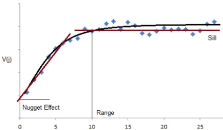
To calculate a variogram, a sufficient number of units (in-crements/samples) are extracted equidistantly, spanning the process interval of interest, or the full transect length, as needed. The variogram is a function of a dimensionless, relative lag parameter, j, which is this distance between two units, the analytical results of which are compared. Full details of the variographic approach are described in DS3077 (2013), Esbensen et al. (2007, 2012a, b), Gy (1998), Minkkinen et al. (2012), and Petersen and Esbensen (2006), Petersen et al. (2005). Variograms may have apparent dif-ferent specific appearances, but three fundamental character-izing features carry all the important information related to sampling errors and the heterogeneity along the transect in any-and-all variogram: the sill, the range, and they axis in-tercept, termed the nugget effect. Definitions of these features are given below.
The sill is theyaxis value at which the variogram levels off and becomes horizontal. The sill represents the total variance calculated from all experimental heterogeneity values. The sill corresponds to the overall maximum variance for the data series if/when calculated without taking their ordering into account.
The range is the lag distance beyond which the variogram v(j) levels off and reaches a stable, constant sill. Samples taken at lags below the range are auto-correlated to a larger and larger degree as the lags become smaller and smaller. The range carries critical information as to the local hetero-geneity with respect to the objective of the present method development.
The nugget effect indicates the amount by which the vari-ance differs from zero when a variogram is extrapolated backwards so as to correspond to what would have been lag =0. A lag equal to zero has no physical meaning, but it represents the hypothetical case of two samples extracted at the same time and location (indeed from exactly the same physical volume of the lot). Thus, although “true replicates” from the exact same soil location (volume) are not physically possible, the nugget effect nevertheless allows for estimation of the corresponding discontinuous variance difference. This can be viewed as a collapse of the 1-D sampling situation (profile, transect) to a stationary sampling situation (small lots, 2-D and 3-D lots); see DS3077 (2013) and Esbensen et al. (2007, 2012a, b) for further descriptions.
The nugget effect has a special interest; it contains all sampling, sample handling/processing, and analytical errors combined, which makes up the total measurement uncer-tainty. A variogram with a high nugget effect with regard to the sill signifies a measurement system not in sufficient control (DS3077, 2013; Esbensen and Wagner, 2014).
necessi-Figure 1.A generic variogram, schematically defining nugget ef-fect, sill, and range. The illustration depicts an increasing vari-ogram, which is the most often occurring type of variogram in the case of significant auto-correlation (for lags below the range) (Kar-danpour et al., 2014). The nugget effect magnitude relative to the sill in this illustration is significant of an acceptable total measurement system,<20 %.
tates outlier deletion after proper recognition and description and occasionally also de-trending of the raw transect data if/when trends are dominant or severe. In this study the raw data transect was de-trended using a simple regression slope subtraction from the data set where needed.
2.3 Mass reduction/subsampling procedure
After the stored samples were thawed and accommodated for 20◦C for a week, before being processed further, the primary field sample size (200–300 g) had to be reduced to the ana-lytical sample size (1–2 g), not at all a trivial mass-handling issue. In order to provide representative subsamples, TOS principles were applied scrupulously to all mass reduction steps. Thus samples were dried and macerated, or ground, where appropriate, and subsequently deployed in a longi-tudinal tray, forming a 1-D lot, using the soil-adapted bed-blending/cross-cut reclaiming technique described in detail in Petersen et al. (2004) and Kardanpour et al. (2015). These pre-blended micro-beds were cut by 10 randomly selected transverse increments along the elongated dimension which were aggregated, resulting in subsamples of 20–30 g each. The exact same procedure was repeated in a secondary mass reduction step further down, ending up with the final analyt-ical mass (2 g) for the wet samples analyses. This procedure has been applied to provide full representativity in samples and to exclude all of the post-primary-sampling errors in or-der to be better able to focus on the latter and the variogram deployment (ibid).
The remainders of the secondary subsamples were air-dried for 4 days at laboratory temperature (20◦C), to be used in parallel sorption experiments. As a further scale-down iter-ation, a similar bed-blending/cross-cut reclaiming was used
to provide analytical samples of 2 g, also based on 10 incre-ments each.
Kardanpour et al. (2015) describe the “from-field-sampling-to-aliquot” pathway in full detail, complete with an exhaustive pictorial presentation.
2.4 Analytical experiment methods
2.4.1 MCPA sorption
The sorption experiment started in glass vials with Teflon caps containing 1 g of the respective soils, and 9 mL of Milli-Q water. The vials were kept for 24 h and then shaken in a horizontal, angled shaker prior to addition of 1 mL14C– MCPA stock solution, with 10 000 dpm in each individual vials. Sorption experiments were performed with two initial concentrations: 1 and 100 mg of MCPA/L. Sorption was de-termined for MCPA in all of the 64 soil samples, using14 C-labelled MCPA.
After adding the stock solution, the vials were incubated in the shaker for 48 h and then placed vertically for another 48 h, all at 20◦C. Subsequently 2 mL of the solution was trans-ferred to the 2 mL Eppendorf micro-centrifuge tubes and centrifuged at 14 500×gfor 7 min. Radioactivity in 1.5 mL of supernatant was determined using a Wallac 1409 liquid scintillation counter after mixing it with 10 mL of OptiPhase Hisafe3 scintillation cocktail.
2.4.2 MCPA mineralization
Mineralization experiments were carried out in a 100 mL glass jar with an airtight lid. Two-gram soil samples (wet weight) were placed in small plastic vials before adding 0.5 mL of14C-labelled MCPA (5 mg MCPA per gram of soil) with a radioactivity of 2000 dpm. A liquid scintillation count-ing (LSC) vial containcount-ing 2 mL of 0.2 M NaOH as a CO2
trap was also placed in the glass jar. The jars were incubated at 20◦C for 14 days. Mineralization encountered as percent-evolved14CO2was measured at day 3, 7, and 14. The CO2
traps were changed and replaced with a fresh trap at each sampling date.14C in the NaOH was measured as described in the sorption experiment by liquid scintillation counting.
2.4.3 Biomass, substrate-induced respiration (SIR)
2.4.4 Microbiology, bacteria colony formation units (CFUs)
A suspension was made with 2 g of soil into 200 mL of ster-ile water, which was then shake for 15 min and diluted with sterilized water; this ended in two different dilutions for each sample, with differences of three and four orders of magni-tude. To measure the soil microbiology, 1 mL of each sam-ple was placed on a Petrifilm®(3M, Saint Paul, Minnesota, USA) sheet and CFUs were counted after 3 and 7 days of incubation at 20◦C.
3 Results
3.1 Geochemical profiling
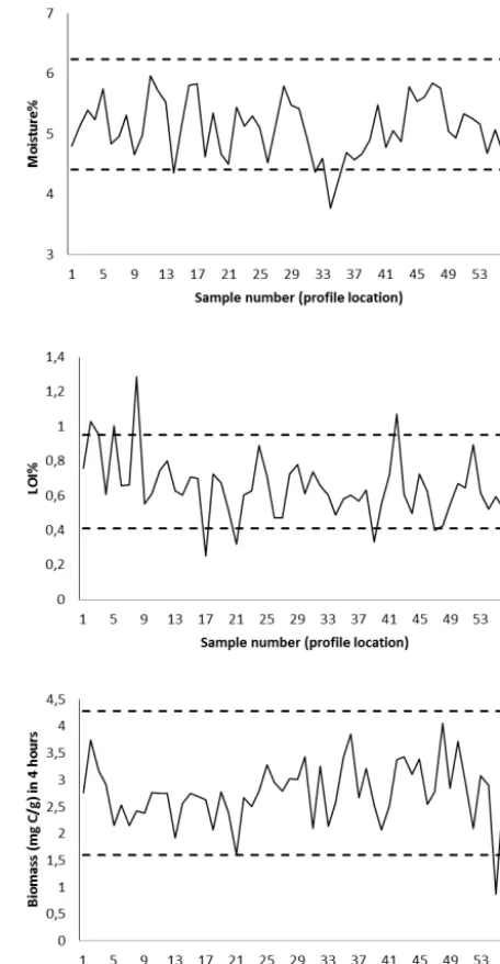
In order to show the natural soil heterogeneity in a compara-ble format, Figs. 2–5 illustrate the individual large-scale pa-rameter transects: concentration vs. location of the samples taken from the transect in the Fladerne field. Also shown is the variation in the central small-scale replication samples is shown as mean concentration±2 SD with dashed horizon-tal lines in the figures. The large-scale variation in the soil moisture, LOI, and the biomass content are compared to the small-scale replication result for the same parameter in each graph (Fig. 2).
The same comparison graph (large scale/small scale) is il-lustrated for the MCPA sorption in Fig. 3 for two different initial MCPA concentrations, as it is clear; the soil sorption behaviour shows different variation with different concentra-tions. The results of the MCPA mineralization of the soil in Fig. 4 also show different variability in different mineraliza-tion steps. The transect of the MCPA mineralizamineraliza-tion is illus-trated for different mineralization steps: the first 3 days, 4 to 7 days, and 8 to 14 days. The two latter periods show a rather similar variation because these two periods are in the final part of the mineralization development (Fig. 6).
The soil microbiology (log (CFU/g soil)) transect after 7 days of incubation is also illustrated in Fig. 5.
The Fladerne case represents an inherently very well mixed soil type, which has been managed by plowing for up to 100 years. The consequence of taking this low-heterogeneity end of the spectrum into account is that there is a limit to the degree of transect heterogeneity to be ex-pected, as indeed witnessed in Figs. 2–5, where concentra-tions only comparatively rarely deviate outside the ±2 SD of the central Roman square design employed. However, this specific soil and tilling history feature must not lead to un-toward confusion and illegitimate generalizations. It is the general applicability of the variographic approach which is illustrated here, as it happens, on a very well mixed substra-tum. Our parallel study showcases the approach on a signifi-cantly more heterogeneous case, in which the central Roman square does not bracket most of the transect concentration manifestations. This case was selected to represent the one
Figure 2.Fladerne Bæk. Transects of soil moisture (%), LOI, and biomass (mg C g−1) vs. soil sample number (transect location). Dashed lines represent mean±2 SD of the small-scale replication experiment.
Figure 3.Fladerne Bæk. Transects ofKdMCPA sorption vs.
sam-ple number (transect location) –Kd,1: MCPA (1 mg L−1);Kd,100:
MCPA (100 mg L−1). Dashed lines represent mean±2 SD of the small-scale replication experiment.
3.2 Experimental variograms
Prior to variogram calculation, all parameters were checked for outliers and trends (Figs. 2–5). Variograms were calcu-lated using large-scale experimental transects without model fitting of the variogram parameters. This is common in geo-statistics but not used here as TOS’ variogram approach is not used for kriging but instead solely for heterogeneity charac-terization and interpretation.
Two different behaviours can be observed as displayed by two parameters groupings: the increasing Min1, LOI, and biomass variograms at the top, versus the remainder of pa-rameters, which show a strongly similar form and behaviour (Fig. 7). As the sill levels represent the maximum parame-ter variation along the transect, parameparame-ters Min1, LOI, and biomass clearly display the highest transect variability. All variograms are of the increasing type with a distinct nugget effect. Following DS3077 (2013), the percentage nugget ef-fect in relation to the sill, termed RSV1-dim, is an expression
of the total measurement uncertainty (MU) including total sampling error (TSE) (Esbensen and Wagner, 2014). In the present study this MUtotal quality index ranges from 15 %
(Kd,100) to 75 % (Min1). There is thus an appreciable
dif-ference concerning the possibility to measure and
character-Figure 4. Fladerne Bæk. Transects of MCPA mineralization in three different periods, i.e. 0–3, 4–7, and 8–14 days, vs. sample number (transect location). Dashed lines represent mean±2 SD of the small-scale replication experiment.
Figure 5.Fladerne Bæk. Transects of log (CFU/g soil) vs. sample number (transect location).
Figure 6.Average mineralization rate for all 57 samples: error bars are based on the standard deviation (solid bars) and the range of the whole sample set (dashed vertical bars).
Through application of the multivariate data analysis ap-proach developed in the previous studies (Kardanpour et al., 2014, 2015), i.e. using the variograms as the input (X ma-trix) to a principal component analysis (PCA) with no cen-tring and no scaling (see further below), the first component is found to represent 99 % of the total variogram variance over all parameters, making it easy to find the average range characterizing the heterogeneity of the Fladerne transect, ca. 5 m. Figure 8 shows the loadings for principal components 1 and 2, displayed in a fashion that mimics a spectrum. As expected, the PC-1 loadings delineate a general variogram shape, in fact presenting the average of all variograms in Fig. 7. The PC-2 loadings account for deviations from here, as caused by the individual variograms (mainly expressing a higher or lower average slope), a general feature that is markedly interprinted by random deviations. This compo-nent models the set of different slopes of the individual var-iograms, and it accounts for less than 1 % total variance, but nevertheless it lends itself easily to interpretation as the well-known spectroscopic “tilting” signature (Martens and Næs, 1991).
Figure 7.Synoptic variogram of all parameters in the present study comparing nugget effect, sill, and range levels.
In our earlier studies (e.g. Kardanpour et al., 2014), a pro et contra discussion can be found regarding pre-treatment of an X matrix made up of variograms. When basing vari-ograms on heterogeneity contributions (a one-to-one trans-formation of the original analytical concentrations), this is-sue becomes moot, as this transformation is already perform-ing what amounts to scalperform-ing. In the present paper we there-fore did not apply centring, opting instead for the easily inter-preted and useful appearance of the average variogram shape (Fig. 8, left).
4 Discussion
Aiming for a general approach to soil heterogeneity char-acterization, a set of naturally occurring organic, anthro-pogenic, and biota parameters were studied at scales from 1 to 60 m to be compared with other, for example minerogenic, parameters (see further below). The first step is always in-spection of the raw data set with respect to potential outliers and/or trends. In the present study the geochemical parameter transects show no outliers and no strong trends (Figs. 2–5).
The experimental design allows comparison of the small-scale replication variability (classic statistics) and large-small-scale variability. All transects can, for example, be directly com-pared with the level and variation at the small-scale experi-ment (less than 1 m), considering the pertinent mean±2 SD. In Figs. 2–5 the variation in the parameters in any selected small-scale window cannot be overestimated to the large scale; indeed, it also cannot be obtained from a small-scale replication study deviation estimate. This is just for visual orientation, however, and not to be confused with the nugget effect, a much more general characterization of the small(est) scale variability pertaining to below lag=1, summing up and averaging this information for all the sample pairs in the transect.
Figure 8.PCA (Xvariogram) loading plot for PC-1 (left) and PC-2 (right). TheXvariogram matrix has not been subjected to pre-treatment
before PCA (no centring, no scaling). The range of the average variogram shape as represented by the PC-1 loadings is ca. 5 m.
variability does not necessarily extend to larger scales. This has an important practical conclusion: no local small-scale sample collection can be generalized to larger scales. Un-witting or unreflected scaling-up of small-scale experimen-tal organic, anthropogenic, and biota fate and mineraliza-tion results will bring an inflated uncertainty outside exper-imental control. The mineralization parameters which show different variation behaviour in the different mineralization steps send an important message regarding studies concern-ing time-dependent characterizations. A similar difference is observed for MCPA sorption with different concentra-tions, i.e. when studies are concerned with concentration-dependent phenomena.
The general local variability behaviour is, however, well captured as the below-range part of the general variogram loading spectrum for PC-1. The variogram is able to gener-alize the common local-scale behaviour. With TOS, there is synoptic information residing in the range, sill, and nugget effect for each individual parameter. Whenever heterogene-ity variograms display a range, this relates to the ease and risk associated with attempting to secure field samples with min-imum variability: sampling with smaller inter-increment lag distances than the range makes it possible to use the inherent auto-correlation between samples in a beneficial fashion.
From the earlier studies (Kardanpour et al., 2014, 2015) the overall conclusion was only to employ composite sam-pling. In the present context this means that, wherever prac-tically possible, increments should only be collected with a maximum of half the observed range as a means to avoid unnecessary compositional variability effects due to the in-herent soil heterogeneity. It follows that, in order to mini-mize the total sampling error, increments must be sampled with a maximum lag of 0.5×range, preferably smaller. In the present soil variograms a general range of 5 m is observed for multivariate variographic approach of the parameters (Fig. 8). It is evident that a thorough mixing of the selected set of increments is mandatory to sample locations with less than 2.5 m distance in between; for other soil types/analytes, other numerical magnitudes apply.
The variograms show different behaviour with respect to mineralization stages. This is expected from the slower rate of the mineralization in the latter stages (Fig. 6). The later
stages display a flat variogram that only represents little auto-correlation between sample locations (Fig. 7) and the low sill level representing low variation along the transect. As is common in environmental studies, results of the mineraliza-tion are mostly reported in terms of the accumulated miner-alization rate (see Fig. 6 as an example), i.e. results that are mostly affected by the first stages of the mineralization.
Most of the variograms level off quickly after only a few lags (range ca. 5 m), followed by a flat (or slightly increasing) trend, whilst the first steps of MCPA mineralization, biomass, and LOI show more markedly increasing variograms (Fig. 7). The CFU sill level is lower than natural organic and an-thropogenic compounds, indicating lower variability in soil microbiology at the large scale(s). This can be compared with results from a series of other large-scale studies on different microbial communities for different anthropogenic and nat-ural compound mineralization, which also showed that mi-crobial biomass seems to be a stable intrinsic parameter of longer periods (Sørensen et al., 2003; Bending et al., 2001, 2003; Walker et al., 2001).
It is always a matter for discussion when theoretically an-ticipated correlations between the physiochemical/microbial activities fail to appear in specific real-world case studies. The more complex compounds have shown a more irregular, patchy fashion of decaying due to more specific microbial communities (but still generally isotropic in nature). Analy-sis of soil parameters rarely gives a clear pattern; this seems to be associated with a number of non-included or unknown parameters, resulting in a high degradation potential in some cases but low elsewhere (Sørensen et al., 2003; Rasmussen et al., 2005; Bending et al., 2001; Walker et al., 2001). Upon reflection, however, this is no mystery but simply a result of local soil heterogeneity, which cannot be formulated or predicted based on the physiochemical biological or micro-bial correlation of the properties of soil in large-scale studies. A variographic heterogeneity characterization at all scales is thus a beneficial pilot experiment able to focus on the rele-vant heterogeneities characterizing individual, or groups of, parameters in their proper scale-dependent relationships.
variographic heterogeneity characterization as a pilot study. Results here will lead to a comprehensive understanding of the spatial variability and auto-correlation of the parameters in the field.
The results from the present study show that, for well-mixed sandy soil, it is recommended to sample locations with less than 2.5 m inter-distance in between, preferably smaller. It is necessary to conduct a similar variographic pilot experi-ment in order to outline the relevant scale-heterogeneity char-acteristics for other soil types, which, unavoidably, will tend to show more irregular spatial heterogeneity patterns – each principal soil type will in principle be characterized by a spe-cific range, but there is a further caveat. Each analyte may in fact display its own more or less specific range, as witnessed above, as well as in a large number of studies in the literature. When controlling the spatial heterogeneity is of the essence, the logical solution is to design the sampling according to the analyte with the smallest range, i.e. the most heteroge-neously distributed analyte – this will by necessity also take care of all other analytes with higher ranges. If the emphasis is on sampling costs, a not completely unlikely alternative scenario that may or may not clash with representativity, it is a comforting thought that all analytes are measured on the same final aliquot. By carefully optimizing the primary field sampling according to the principles presented here, all an-alytes will be measured with the same, optimal relevance, indeed with regard to the same representativity. If sampling is done right from the start, there are no extra costs – the op-posite, however, is a very different case, as should be abun-dantly clear.
Results from a parallel study on the minerogenic com-pounds for the same Fladerne field (Kardanpour et al., 2014) show a similar soil heterogeneity compared to the present anthropogenic compounds. The nugget effects for most of the minerogenic compounds are of the same or-der of magnitude as those for the anthropogenic compounds – i.e. the total measurement system and procedures (sam-pling/handling/processing/analysis) pass all the quality crite-ria for representative sampling established in the recent sam-pling standard (DS3077, 2013).
In cases where the next step in studies might be assess-ment of the main factors driving the spatial heterogeneity of soil contamination analytes, for example, the 1-D (or 2-DX−Y) approach advocated here will only serve as a basis for proper selection of experimental material to be taken to the laboratory – upon which further considerations will fo-cus on, say, the potential factors involved in contaminant in-put and transport, among other things. Note that these latter processes manifest themselves primarily in theZ direction, where it is by no means a given that application of the same variographic approach (or geostatistical modelling) will nec-essary give meaningful results.
5 Conclusions
A pilot experiment aimed at an intrinsic 1-D soil heterogene-ity characterization is a critical success factor for laboratory studies relying on field samples to provide the experimental pots, which for replicate and comparative study objectives need to be as similar as at all possible. As a case study, the variographic results for sandy soils show that the distance between two sample spot must be less than 2.5 m for the present set of organic compounds and soil type. Specific soil types and/or other analytes will in principle display differ-ent ranges and nugget effects, and hence our call for system-atic deployment of the variographic pilot experiment, from which all necessary information can be derived for designing an optimal sampling plan, e.g. identifying the analyte with the smallest range (for significantly correlated analytes). For the case of well-mixed soil components, a general PCA ap-proach for modelling a whole set of variograms may be use-ful in addition to individual analyte consideration.
Without these types of information, experimental fate study work is essentially devoid of a valid basis as regards interpretation, scaling up, and scientific generalization of the experimental results back to the field scale. A large-scale 1-D transect sampling can reveal the inherent heterogeneity at all scales, from the smallest local sampling equidistance up to the maximum experimental length scale studied. Vario-graphic analysis was here employed successfully to soil het-erogeneity at scales between 1 and 100 m; other scenarios may require other numerical parameters, while the general approach remains identical.
The TOS-guided variogram pilot study approach illus-trated here has a substantial carrying-over potential to geo-chemistry and environmental science, as well as other areas of application. It is even applicable to dynamic systems, i.e. to natural or technological processes in these realms.
Acknowledgements. The authors gratefully acknowledge the Danish Research Council for PhD stipend funding (stipend no. 562/06-18-10028(6)) to Z. Kardanpour and valuable laboratory services and assistance provided by GEUS, Dept. of Geochemistry. The authors are grateful to GEUS’ management for a positive attitude with respect to development and application of TOS’ principles of proper representative sampling, which are not always recognized in geoscience communities.
References
Adamchuk, V. I., Viscarra Rossel, R. A., Marx, D. B., and Samal, A. K.: Using Targeted Sampling to Process Multivariate Soil Sens-ing Data, Geoderma, 163, 63–73, 2011.
Arias-Estévez, M., López-Periago, E., Martínez-Carballo, E., Simal-Gándara, J., Mejuto, J.-C., and García-Río, L.: The Mo-bility and Degradation of Pesticides in Soils and the Pollution of Groundwater Resources, Agr. Ecosyst. Environ., 123, 247–260, 2008.
Bending, G., Shaw, E., and Walker, A.: Spatial Heterogeneity in the Metabolism and Dynamics of Isoproturon Degrading Microbial Communities in Soil, Biol. Fert. Soils, 33, 484–489, 2001. Bending, G. D., Lincoln, S. D., Sebastian, R., Morgan, J. A. W.,
Aamand, J., Sørensen, S. R., and Walker, A.: In-Field Spatial Variability in the Degradation of the Phenyl-Urea Herbicide Iso-proturon Is the Result of Interactions between Degradative Sph-ingomonas Spp. and Soil pH, App. Environ. Microbiol., 69, 827– 834, 2003.
Boudreault, J.-P., Dubé, J.-S., Sona, M., and Hardy, E.: Analysis of Procedures for Sampling Contaminated Soil Using Gy’s Sam-pling Theory and Practice, Sci. Total Environ., 425, 199–207, 2012.
Chappell, A. and Viscarra Rossel, R. A.: The Importance of Sam-pling Support for Explaining Change in Soil Organic Carbon, Geoderma, 193–194, 323–325, 2013.
Crespin, M. A., Gallego, M., Valcárcel, M., and González, J. L.: Study of the Degradation of the Herbicides 2,4-D and MCPA at Different Depths in Contaminated Agricultural Soil, Environ. Sci. Technol., 35, 4265–4270, 2001.
De Zorzi, P., Barbizzi, S., Belli, M., Fajgelj, A., Jacimovic, R., Jeran, Z., Sansone, U., and van der Perk, M.: A Soil Sampling Reference Site: The Challenge in Defining Reference Material for Sampling, Appl. Radiat. Isotopes, 66, 1588–1591, 2008. Dictor, M.-C., Tessier, L., and Soulas, G.: Reassessment of theK
EC Coefficient of the Fumigation±Extraction Method in a Soil Profile, Soil Biol. Biochem., 30, 119–127, 1998.
DS3077: Representative Sampling/ Horizontal Standard, Danish Standard Authority, 44, 1–38, 2013.
Esbensen, K. H. and Romanach, R. J.: Counteracting soil hetero-geneity sampling for environmental studies (pesticide residues, contaminants transformation) – TOS is critical, Proceedings 7th World Conference on Sampling and Blending (WCSB7), 205– 209, 2015.
Esbensen, K. H. and Wagner, C.: Theory of Sampling (TOS) versus Measurement Uncertainty (MU) – A Call for Integration, TrAC-Trend. Anal. Chem., 57, 93–106, 2014.
Esbensen, K. H., Friis-Petersen, H. H., Petersen, L., Holm-Nielsen, J. B., and Mortensen, P. P.: Representative Process Sampling – in Practice: Variographic Analysis and Estimation of Total Sam-pling Errors (TSE), Chemometr. Intell. Lab., 88, 41–59, 2007. Esbensen, K. H., Paoletti, C., and Minkkinen, P.: Representative
Sampling of Large Kernel Lots I. Theory of Sampling and Var-iographic Analysis, TrAC-Trend. Anal. Chem., 32, 154–164, 2012a.
Esbensen, K. H., Paoletti, C., and Minkkinen, P.: Representative Sampling of Large Kernel Lots III. General Considerations on Sampling Heterogeneous Foods, TrAC-Trend. Anal. Chem., 32, 178–184, 2012b.
Gerlach, R. W., Dobb, D. E., Raab, G. A., and Nocerino, J. M.: Gy Sampling Theory in Environmental Studies. 1. Assessing Soil Splitting Protocols, J. Chemometr., 16, 321–328, 2002. Gy, P. M.: Sampling for Analytical Purposes, 1st Edn. Chichester,
West Sussex, UK, John Wily & Sons, 172 pp., ISBN: 978-0-471-97956-2, 1998.
Johnsen, A. R., Styrishave, B., and Aamand, J.: Quantifica-tion of Small-Scale VariaQuantifica-tion in the Size and ComposiQuantifica-tion of Phenanthrene-Degrader Populations and PAH Contaminants in Traffic-Impacted Topsoil, FEMS Microbiol. Ecol., 88, 84–93, 2014.
Kardanpour, Z., Jacobsen, O. S., and Esbensen, K. H.: Soil Het-erogeneity Characterization Using PCA (Xvariogram) – Multi-variate Analysis of Spatial Signatures for Optimal Sampling Pur-poses, Chemometr. Intell. Lab., 136, 24–35, 2014.
Kardanpour, Z., Jacobsen, O. S., and Esbensen, K. H.: Counteract-ing soil heterogeneity samplCounteract-ing for environmental studies (pes-ticide residues, contaminants transformation) – TOS is critical, Proceedings 7th World Conference on Sampling and Blending (WCSB7), 205–209, 2015.
Li, B. G., Cao, J., Liu, W. X., Shen, W. R., Wang, X. J., and Tao, S.: Geostatistical Analysis and Kriging of Hexachlorocyclohexane Residues in Topsoil from Tianjin, China, Environ. Pollut., 142, 567–575, 2006.
Lin, Q., Li, H., Luo, W., Lin, Z., and Li, B.: Optimal Soil-Sampling Design for Rubber Tree Management Based on Fuzzy Cluster-ing, Forest Ecol. Manage., 308, 214–222, 2013.
Martens, H. and Næs, T.: Multivariate Calibration, John Wiley & Sons, Chichester, West Sussex, UK, 438 pp., ISBN: 978-0-471-93047-1, 1991.
Minkkinen, P., Esbensen, K. H., and Paoletti, C.: Representative Sampling of Large Kernel Lots II. Application to Soybean Sam-pling for GMO Control, TrAC-Trend. Anal. Chem., 32, 165–177, 2012.
Mulder, V. L., de Bruin, S., and Schaepman, M. E.: Representing Major Soil Variability at Regional Scale by Constrained Latin Hypercube Sampling of Remote Sensing Data, Int. J. Appl. Earth Obs., 21, 301–310, 2013.
Petersen, L. and Esbensen, K. H.: Representative Process Sampling for Reliable Data Analysis — a Tutorial, J. Chemometr., 19, 625– 647, 2006.
Petersen, L., Dahl, C. K., and Esbensen, K. H.: Representative Mass Reduction in Sampling – a Critical Survey of Techniques and Hardware, Chemometr. Intell. Lab., 74, 95–114, 2004.
Petersen, L., Minkkinen, P., and Esbensen, K. H.: Representa-tive Sampling for Reliable Data Analysis: Theory of Sampling, Chemometr. Intell. Lab., 77, 261–277, 2005.
Rasmussen, J., Aamand, J., Rosenberg, P., Jacobsen, O. S., and Sørensen, S. R.: Spatial Variability in the Mineralisation of the Phenylurea Herbicide Linuron within a Danish Agricultural Field: Multivariate Correlation to Simple Soil Parameters, Pest Manage. Sci., 61, 829–837, 2005.
Rodriguez-Cruz, M. S., Jones, J. E., and Bending, G. D.: Field-Scale Study of the Variability in Pesticide Biodegradation with Soil Depth and Its Relationship with Soil Characteristics, Soil Biol. Biochem., 38, 2910–2918, 2006.
Het-erogeneity Impact MCPA Degradation in and Leaching from a Loamy Agricultural Soil?, Sci. Total Environ., 472, 90–98, 2014. Sørensen, S. R., Bending, G. D., Jacobsen, C. S., Walker, A., and Aamand, J.: Microbial Degradation of Isoproturon and Related Phenylurea Herbicides in and below Agricultural Fields, FEMS Microbiol. Ecol., 45, 1–11, 2003.
Sørensen, S. R., Schultz, A., Jacobsen, O. S., and Aamand, J.: Sorption, Desorption and Mineralisation of the Herbicides Glyphosate and MCPA in Samples from Two Danish Soil and Subsurface Profiles, Environ. Pollut., 141, 184–194, 2006. Tate, K. R., Ross, D. J., and Feltham, C. W.: A Direct Extraction
Method to Estimate Soil Microbiology C: Effects of Experimen-tal Variables and Some Different Calibration Procedures, Soil Biol. Biochem., 20, 329–335, 1988.
Torstensson, N. T. L. and Stark, J.: The Effect of Repeated Appli-cations of 2, 4-D and MCPA on Their Breakdown in Soil, Weed Res., 15, 159–164, 1975.
Totaro, S., Coratza, P., Durante, C., Foca, G., Li Vigni, M., Marchetti, A., Marchetti, M., and Cocchi, M.: Soil Sampling Planning in Traceability Studies by Means of Experimental De-sign Approaches, Chemometr. Intell. Lab., 124, 14–20, 2013. Walker, A., Jurado-Exposito, M., Bending, G. D., and Smith, V. J.: