www.earth-syst-dynam.net/7/211/2016/ doi:10.5194/esd-7-211-2016
© Author(s) 2016. CC Attribution 3.0 License.
Projections of leaf area index in earth system models
Natalie Mahowald1, Fiona Lo1, Yun Zheng1, Laura Harrison2, Chris Funk2, Danica Lombardozzi3, and Christine Goodale4
1Department of Earth and Atmospheric Sciences, Cornell University, Ithaca, NY 14853, USA 2Department of Geography, University of California at Santa Barbara, Santa Barbara, CA 93106, USA 3Climate and Global Dynamics Division, National Center for Atmospheric Research, Boulder, CO 80307, USA
4Department of Ecology and Evolutionary Biology, Cornell University, Ithaca, NY 14853, USA Correspondence to: Natalie Mahowald ([email protected])
Received: 3 March 2015 – Published in Earth Syst. Dynam. Discuss.: 15 April 2015 Revised: 22 February 2016 – Accepted: 25 February 2016 – Published: 9 March 2016
Abstract. The area of leaves in the plant canopy, measured as leaf area index (LAI), modulates key land– atmosphere interactions, including the exchange of energy, moisture, carbon dioxide (CO2), and other trace gases and aerosols, and is therefore an essential variable in predicting terrestrial carbon, water, and energy fluxes. Here our goal is to characterize the LAI projections from the latest generation of earth system models (ESMs) for the Representative Concentration Pathway (RCP) 8.5 and RCP4.5 scenarios. On average, the models project increases in LAI in both RCP8.5 and RCP4.5 over most of the globe, but also show decreases in some parts of the tropics. Because of projected increases in variability, there are also more frequent periods of low LAI across broad regions of the tropics. Projections of LAI changes varied greatly among models: some models project very modest changes, while others project large changes, usually increases. Modeled LAI typically increases with modeled warming in the high latitudes, but often decreases with increasing local warming in the tropics. The models with the most skill in simulating current LAI in the tropics relative to satellite observations tend to project smaller increases in LAI in the tropics in the future compared to the average of all the models. Using LAI projections to identify regions that may be vulnerable to climate change presents a slightly different picture than using precipitation projections, suggesting LAI may be an additional useful tool for understanding climate change impacts. Going forward, users of LAI projections from the CMIP5 ESMs evaluated here should be aware that model outputs do not exhibit clear-cut relationships to vegetation carbon and precipitation. Our findings underscore the need for more attention to LAI projections, in terms of understanding the drivers of projected changes and improvements to model skill.
1 Introduction
Providing future projections of climate change feedbacks and impacts is one of the goals motivating the development of earth system models (ESMs). The latest generation of ESMs includes land models that simulate the temporal evolution of carbon and vegetation (Friedlingstein et al., 2006). To do so, these models predict leaf area index (LAI) and other carbon cycle variables. LAI represents the amount of leaf area per unit land area, and is an important land carbon at-tribute. Many ESMs calculate leaf-level carbon and water fluxes, which are then scaled regionally and globally based
cou-pled models (e.g., Randerson et al., 2009; Luo et al., 2012, Anav et al., 2013b). Finally changes in LAI, and the related normalized difference vegetation index (NDVI), can indicate ecosystem health and natural resource availability. As such, LAI is used within the famine prediction community (Funk and Brown, 2006; Groten, 1993) and represents a variable that is easy to use in climate impacts studies. Thus it is im-portant to consider the 21st century projections for LAI in earth system models.
The current generation of ESMs has prepared historical and future scenario simulations within the Coupled Modeling Intercomparison Project (CMIP5) (Taylor et al., 2009). There have been extensive evaluations and comparisons of the fu-ture projections of the land, ocean, and atmospheric carbon cycle in the ESMs in the CMIP5 (e.g., Arora et al., 2013; Friedlingstein et al., 2013; Jones et al., 2013). There has also been comparison of ESM-simulated seasonal variability in LAI against satellite-based observations for the high latitudes (Anav et al., 2013a; Murray-Tortarolo et al., 2013), as well as comparisons of LAI and other variables in ESMs across the globe (Anav et al., 2013b). Additionally, Shao et al. (2013), Mao et al. (2013), and Sitch et al. (2015) evaluated the rela-tionship between the carbon cycle and other variables, such as temperature, or LAI, over decadal and longer timescales. These ESM-based comparisons build on the long history of evaluation of model simulations of vegetation properties and carbon balance (e.g., Cramer et al., 1999).
Here, our goal is to characterize the ESM projections of fu-ture LAI in order to better understand how LAI is projected to change. Most of our analysis emphasizes the Represen-tative Concentration Pathway (RCP) 8.5, the most extreme future scenario, and we contrast it with RCP4.5, a less ex-treme scenario (van Vuuren et al., 2011) (Sect. 3). We char-acterize both the model mean LAI projected change, as well as the model mean divided by the standard deviation (e.g., Meehl et al., 2007; Tebaldi et al., 2011). In addition, we con-sider whether LAI projections can help the climate impact community anticipate regions that may experience increased climate exposure and increased risk of food insecurity in the future. Changes in LAI variability are also important for un-derstanding the impact of climate change, since they can lead to an increase in the length and frequency of low LAI events, even as mean LAI increases. We consider, therefore, both changes in the mean and the frequency of low LAI events, and how this information compares to precipitation projec-tions, which are commonly used for climate impact studies (e.g., Field et al., 2014). We also consider what model traits may be related to the spread in the future model projections (Sect. 3). We use evaluations of LAI, based on satellite-based observations (e.g., Zhu et al., 2013; Anav et al., 2013b; Sitch et al., 2015), to characterize the relationship between model skill and projections (e.g., Steinacher et al., 2010; Cox et al., 2013; Flato et al., 2013; Hoffman et al., 2014) (Sect. 4). Section 5 presents our summary and conclusions.
2 Methods and data sets
2.1 Model data sets
Coupled carbon model experiments were included as part of the CMIP5 experiments (e.g., Arora et al., 2013; Tay-lor et al., 2009). The historical simulations and Representa-tive Concentration Pathway for 8.5 (RCP8.5; van Vuuren et al., 2011; Riahi et al., 2011), using prescribed carbon dioxide concentrations, were analyzed here (Table 1). We chose to fo-cus on the RCP8.5 scenario as it has the largest changes in carbon dioxide and climate. Analysis of the RCP4.5 scenario (Wise et al., 2009; van Vuuren et al., 2011) is also included for comparison for the models which included the RCP4.5 simulations at the CMIP5 archive (all models except BNU-ESM and CBNU-ESM-BGC).
Model variables analyzed included monthly-mean precip-itation, near-surface air temperature, vegetation carbon stock and LAI. Only models which had data for all these variables for both historical and RCP8.5 scenarios were included in this study. Some models submitted multiple versions, at dif-ferent resolutions or with slightly difdif-ferent physics (Table 1). Even though some of the models are closely related (e.g., CESM1-BGC and NorESM-ME), we include different con-figurations of the same model.
2.2 Model future projection analysis
This analysis examines model mean changes between the current climate (1981–2000) and future climate time peri-ods (2011–2030, 2041–2060 and 2081–2100). To identify the location where models project statistically significant changes, we analyze the ratio of the mean change to vari-ability; this is accomplished by dividing the mean changes over 20-year time periods by the standard deviation over the current climate (1981–2000) and shown in terms of stan-dard deviation units (e.g., Mahlstein et al., 2012; Tebaldi et al., 2011). Previous studies have shown that the spatial and temporal scale used to define these changes can determine whether these signals are statistically significant (Lombar-dozzi et al., 2014). We focus on three time periods through-out the 21st century because the change in LAI can poten-tially switch between positive and negative in these different time periods (e.g., Lombardozzi et al., 2014), and we want to identify whether the changes through time are gradual, or if there is a tipping point.
Table 1.Model simulations from the Climate Modeling Intercomparison Projection (CMIP5) included in this study. All models listed here were available for the RCP8.5 analysis, while all models except BNU-ESM and CESM-BGC were available for the RCP4.5 analysis.
Model Land model Land N- Dynamic Citation
resolution cycle veg.
BCC-CSM1 BCC-AVIM1.0 2.8◦×2.8◦ N Y Wu et al. (2013)
BCC-CSM1-M BCC-AVIM1.0 1.1◦×1.1◦ N Y Wu et al. (2013)
BNU-ESM CoLM+BNU-DGVM 2.8◦×2.8◦ N Y BNU-ESM,
http://esg.bnu.edu.cn
CanESM2 CLASS2.7+CTEM1 2.8◦×2.8◦ N N Arora et al. (2011)
CESM1-BGC CLM4 0.9◦×1.2◦ Y N Lindsay et al. (2014)
GFDL-ESM2G LM3 2.5◦×2.5◦ N Y Dunne et al. (2013)
GFDL-ESM2M LM3 (uses different physical ocean model) 2.5◦×2.5◦ N Y Dunne et al. (2013)
HadGEM2-CC JULES+TRIFFID 1.9◦×1.2◦ N Y Collins et al. (2011)
HadGEM2-ES JULES+TRIFFID (includes chemistry) 1.9◦×1.2◦ N Y Collins et al. (2011)
INM-CM4 Simple model 2◦×1.5◦ N N Volodin et al. (2010)
IPSL-CM5A-LR ORCHIDEE 3.7◦×1.9◦ N N Dufresne et al. (2013)
IPSL-CM5A-MR ORCHIDEE 2.5◦×1.2◦ N N Dufresne et al. (2013)
IPSL-CM5B-LR ORCHIDEE (improved parameterization) 3.7◦×1.9◦ N N Dufresne et al. (2013)
MIROC-ESM_ MATSIRO+SEIB-DGVM 2.8◦×2.8◦ N Y Watanabe et al. (2011)
MIROC-ESM-CHEM MATSIRO+SEIB-DGVM adds chemistry) 2.8◦×2.8◦ N Y Watanabe et al. (2011)
MPI-ESM-LR JSBACH+BETHY 1.9◦×1.9◦ N Y Raddatz et al. (2007)
MPI-ESM-MR JSBACH+BETHY (ocean model higher resolution) 1.9◦×1.9◦ N Y Raddatz et al. (2007)
NorESM1-ME CLM4 2.5◦×1.9◦ Y N Bentsen et al. (2013)
use this metric to estimate the fraction of the time in the fu-ture that this condition exists, and specifically whether it in-creases in the future.
2.3 Observational data
LAI data derived from satellite over the 30-year period 1981– 2010 are used to evaluate the CMIP5 model skill in the cur-rent climate. This observational data set is derived using neu-ral network algorithms using the Global Inventory Modeling and Mapping (GIMMS) Normalized Difference Vegetation Index (NDVI3g) and the Terra Moderate Resolution Spec-troradiometer (MODIS) LAI (Zhu et al., 2013). The satel-lite data are only available over regions with green vegeta-tion, and thus are lacking over desert and arid regions. A de-tailed description of the algorithm and comparison to ground-truth observations are shown in Zhu et al. (2013). Compared with field-measured LAI, mean squared errors (RMSE) in the satellite LAI estimates are estimated to be approximately 0.68 LAI, for spanning LAI ranges from<1 to almost 6 (Zhu et al., 2013). Comparisons with ground-based observations confirm that the new LAI product also seems to capture ob-served interannual variability patterns (Zhu et al., 2013).
Gridded temperature data for the period 1981–2010 were derived from the Global Historical Climatology Network and Climate Anomaly Monitoring System (GHCN_CAMS) 2 m temperature data set (Fan and van den Dool, 2008). Estimates of the uncertainty in temperature gridded data sets suggest that the uncertainty in temperatures at a grid box level is es-timated to be between 0.2 and 1◦C (Jones et al., 1997; Fan and van den Dool, 2008).
2.4 Methodology for evaluation of current climate LAI simulation
Several recent studies have used the same new satellite-derived LAI data set (GIMMS LAI3g) in land model evaluation (e.g., Murray-Tortarolo et al., 2013; Anav et al., 2013a, b; Mao et al., 2013; Sitch et al., 2015), includ-ing some of the same land models used here. Thus we do not repeat a complete evaluation of model LAI compared to satellite LAI. We use the satellite LAI data set to consider whether there is a relationship between the models’ ability to simulate LAI in the current climate and the models’ cli-mate projections. We use a few basic metrics in this study (Table 2), which are described briefly below.
Results for the model and observations are evaluated on a 2.5◦×2.5◦ grid based on the observed temperature data grid (see Sect. 2.3). For the metric analysis here, the aver-ages shown are grid-box means, not areal averaver-ages. This al-lows us to use similar weighting for both the averages and the rank correlation coefficients, and tends to weight the global analysis towards high latitudes. However, most of the analy-sis focuses on regional areas (tropical (<30◦), mid-latitudes (>30 and<60◦) and high-latitudes (>60◦), where the dif-ferences between weighting by area and weighting by grid box are reduced.
observa-Table 2.Table of metrics for LAI comparisons between model and observation used in the following tables. More description of these metrics are provided in Sect. 2.4.
Metrics Description
Mean Model/obs Ratio of mean LAI from the model and observations Corr. Spatial correlation of mean LAI
SD seasonal
Model/obs Ratio of seasonal cycle strength: ratio of standard deviation of the climatological monthly mean LAI from the model and observations
Avg. Corr. Avg. Corr. of the temporal evolution of the climatological seasonal cycle in the model vs. observations at each grid box
SD IAV Model/obs Ratio of IAV strength: ratio of standard deviation of the annual mean LAI from the model and observations
IAV LAI vs. T Avg. Corr. Avg. Corr. between LAI and temperature in IAV
IAV LAI vs date Avg. Corr. Avg. Corr. between LAI and date in IAV
tions are averaged and compared over different areas: global, tropical (<30◦), mid-latitudes (>30 and<60◦) and high-latitudes (>60◦) (Table 2: mean LAI: model/obs.). A second metric evaluates the models’ ability to capture spatial vari-ations in LAI, using the spatial correlation across the grid-boxes of the annual mean LAI in the model compared to the observations (e.g., Anav et al., 2013b; Table 2: Mean: Corr.). Important for this study is the consideration of the tempo-ral variability simulated in the model. The magnitude of the seasonal cycle is calculated as the standard deviation of the climatological monthly means at each grid box. This met-ric is slightly different than how LAI has previously been evaluated in some studies (e.g., Anav et al., 2013a; Murray-Tortarolo et al., 2013; Sitch et al., 2015), but is more similar to analyses of other climate variables (Gleckler et al., 2008), facilitating inclusion of LAI within climate model evalu-ations. Metrics for the seasonal cycle were computed us-ing a spatial average over each region (Table 2: SD Sea-sonal: Model/obs). For the seasonal cycle, the ability to cap-ture the timing of phenology can be important (e.g., Anav et al., 2013a; Zhu et al., 2013). To analyze this ability, we computed the temporal correlation of observed and model-simulated monthly means at every grid box, and then aver-aged over each region (Table 2: Seasonal Avg. Corr.).
To evaluate the models’ ability to simulate LAI interannual variability (IAV), we consider the magnitude of the interan-nual variability, which is calculated as the standard deviation of annual mean LAI across years at each grid box (e.g., Zhu et al., 2013). The IAV is then spatially averaged and com-pared between the model and satellite observations (Table 2: SD IAV: Model/obs.). We focus our study on IAV, based on the inter-annual means, but there may be important changes in the seasonal cycle or length of growing season on an inter-annual time basis, which our simple approach does not con-sider (e.g., Murray-Tortarolo et al., 2013).
Previous studies have examined correlations between tem-perature and satellite-derived LAI (e.g., Anav et al., 2013a, b; Zhu et al., 2013) or the closely related normalized
differ-ence vegetation index (NDVI; Zeng et al., 2013). Observed variations of LAI at high latitudes tend to be dominated by changes in temperature, while the tropics are more domi-nated by moisture (Anav et al., 2013a, b; Zeng et al., 2013), which is also seen in coupled carbon climate models for car-bon cycle variables (e.g., Fung et al., 2005). In order to un-derstand what may be driving the IAV in the LAI, we calcu-late metrics to examine the rank correlation between anoma-lies in LAI and anomaanoma-lies in temperature and trends with time. Although correlations do not identify causation, they can help identify the strength of relationships among various driving factors.
This analysis focuses on the relationship between temper-ature and LAI for comparing interannual variability in the modeled and observed data sets. Sensitivity studies have in-dicated that the grid-box level relationship between temper-ature and LAI is a good indicator of fetemper-atures intrinsic to the model, rather than to the meteorology forcing the model (Fig. S1 in the Supplement; as seen also in Anav et al., 2013a; Murray-Tortarolo et al., 2013). This was not the case for the relationship between precipitation and LAI. In sensitiv-ity studies conducted as part of this study, we forced the Community Land Model (Lawrence et al., 2012; Lindsay et al., 2014), which is the land model used in the CESM (Ta-ble 1), with reanalysis-derived data combined with observed precipitation (Qian et al., 2006; Harris et al., 2013) instead of model derived meteorology. The LAI-precipitation relation-ship across IAV was very sensitive to the meteorology used, and thus is not shown or used to evaluate the current climate simulations of LAI (Fig. S1). This implies that errors in the simulations of the mean and variability in precipitation in the current climate, which are very difficult for ESMs to simu-late well (e.g., Flato et al., 2014), are very important for the simulation of IAV in LAI.
our model evaluation, we exclude grid boxes with more than 50 % of agricultural land use based on Ramankutty et al. (2008). Results of the model evaluation with and without agricultural grid-box were quantitatively and qualitatively similar to those presented here, and thus we include all grid-boxes in this analysis. Future simulations are unlikely to be more sensitive than the historical simulations to land use and land cover change, because the scenarios include less future land cover change than that which has occurred historically (Hurtt et al., 2011; Van Vuuren et al., 2011).
For ease of interpretation, we present the metrics described above in Fig. 9, in which higher numbers represent a better simulation. For correlations, this representation is straight-forward: 1 is a perfect correlation and lower values repre-sent a worse simulation. For the other metrics that are not correlations, we convert the statistics to values with similar ranges to facilitate ease of display. The mean model bias met-ric (model/obs) is normalized to a value that varies between 0 and 1, with 1 being close to the observed data. This approach penalizes models which have too high of a mean equally with model that have too low of a mean, using the following for-mula (Fig. 9):
Model Evaluation Value= 2
n
Model Mean
Observed Mean+
Observed Mean Model Mean
o. (1)
We use this method to convert mean biases and standard deviation biases to a model evaluation value (MEV). This is a slightly different method than used in previous studies (e.g., Gleckler et al., 2008), as the MEV does not square the stan-dard deviations. Since we use ranks and rank correlations, the difference between these methods is unlikely to be im-portant, and allows us to use a similar ranking method for mean and standard deviation comparisons.
3 Results
3.1 Future projections
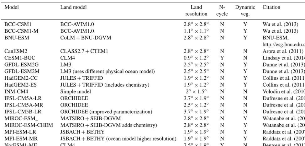
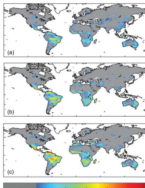
First we consider the model mean projections of change in LAI for RCP8.5, similar to analyses for other standard model variables, and show their evolution through the 21st century (e.g., Meehl et al., 2007). Across most of the globe, LAI is projected to increase through 2081–2100, with small de-creases projected for parts of Central and South America and Southern Africa (Fig. 1). The increases in LAI are largest in high latitudes, mountainous regions (e.g., Tibetan plateau) and some parts of the mid-latitudes and tropics (Fig. 1; for reference, mean satellite observed LAIs in the current cli-mate are presented in Fig. S2). Notice that in this study we use projections of human land use based on the RCP8.5 or RCP4.5, and thus an important human role in future land cover change is driven by the assumptions of the scenario chosen for these studies. Generally, for all the RCPs, there is less land use and land cover change projected in the
fu-Figure 1. Mean of all models for the annual mean change in LAI (m2m−2) over time relative to current (1981–2000) for 2011– 2030 (a), 2041–2060 (b) and 2081–2100 (c) for RCP8.5.
ture than what has occurred in the past (e.g., van Vuuren et al., 2011; Ward et al., 2014).
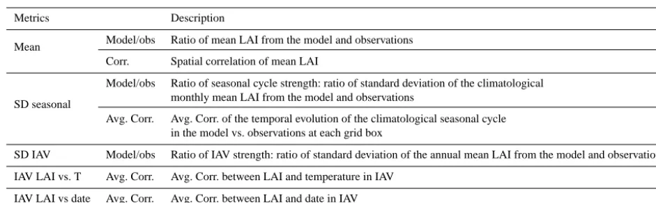
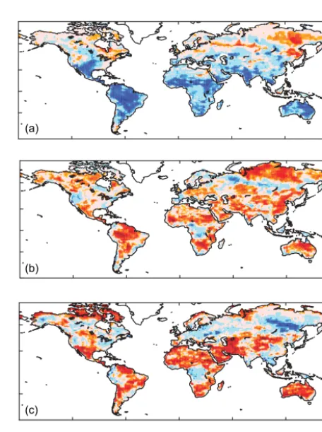
In order to isolate the changes that are statistically sig-nificant, for each model we divided the change in LAI by the IAV standard deviation. Values over 1 are considered statistically significant (e.g., following Tebaldi et al., 2011; Mahlstein et al., 2012). Using this approach, statistically sig-nificant changes in LAI start over the high latitudes, and spread over much of the globe with time (Fig. 2). By 2081– 2100, the increases in LAI are 8 times as large as IAV over large parts of high-latitude regions, as well as the Tibetan plateau and some desert regions, indicating large changes (Fig. 2c). Part of the reason for these very large normalized LAI values is that they have low IAV in the current climate. A few isolated tropical regions are projected to have statisti-cally significant reductions in mean LAI, such as in Central America and the Amazon basin.
Figure 2. Mean of all models for the annual mean change in LAI over time relative to current (1981–2000), normalized by each model’s current (1981–2000) standard deviation at each grid point, for 2011–2030 (a), 2041–2060 (b) and 2081–2100 (c) for RCP8.5.
Mitchell, 2003; Moss et al., 2010). There is a consistent rela-tionship between changes in LAI and temperature across the different time periods for each model; that is, most models and regions show a constant slope between changes in LAI and temperature (Fig. 3). Most models even show a similar slope between LAI and temperature for the RCP4.5 as the RCP8.5 (Fig. S4). Recognize that the change in temperature scales with the change in CO2forcing from carbon dioxide fertilization as well as other physical variables such as pre-cipitation (e.g., Mitchell, 2003; Moss et al., 2010). This sim-ilarity in slope for each model across RCPs and time periods breaks down in the tropics for a few of the models, as some show steeper increases in LAI at warmer temperatures and others shift from LAI increases to declines as warming con-tinues (GFDL, IPSL, MIROC and MPI models) (Fig. 3b). Across the tropics, LAI is projected to increase in some re-gions and decrease in others, so small changes in the rela-tive area of these changes can lead to large shifts in the re-gional net mean LAI change. The value of spatial correla-tions between the RCP4.5 and RCP8.5 mean LAI change at each gridbox for the 2081–2100 time period is 0.81, 0.70, 0.79 and 0.89, for the globe, tropics, mid-latitudes and high-latitudes, respectively (averaged across the models), showing the spatial coherence in the LAI projections between these two RCPs. Even the models with the lowest spatial
corre-lations between the two RCPs (GFDL, IPSL, MIROC and MPI) have statistically significant correlation coefficients of 0.45 or higher in the tropics, where correlations are the low-est.
The models project a wide range of future changes in LAI (Fig. 3). One model (BNU-ESM) projects a large global mean increase of over 1 m2m−2by 2081–2100. For the other models, projected global mean increases in LAI amounted to 0.5 m2m−2 or less. Some models (inmcm4, IPSL, MIROC and MPI model versions) projected small net decreases in LAI in the tropics (Fig. 3). Inter-model differences become even more apparent at the grid-box level, with very different changes in LAI projected by the different models (Fig. S5). The spread in model projections is discussed further below (Sect. 4) in relation to whether there is a relationship between model skill at predicting LAI in the current climate and fu-ture model projections (e.g., Steinacher et al., 2010; Flato et al., 2013; Cox et al., 2013; Hoffman et al., 2014).
3.2 Identifying regions at risk due to climate change
(a) Global (b) Tropics
1.5
1.0
0.5
0 0
0 1.5
1.0
0.5
0
LA
I (
m
m
)
2
–2
Δ
2 ΔTemp (C)4 6 0 2 ΔTemp (C)4 6
(c) Mid-Lat. (d) High-Lat.
1.5
1.0
0.5
0
1.5
1.0
0.5
0
0 2 ΔTemp (C)4 6
2 ΔTemp (C)4 6
A B C D E
F G H I J
K L M N O
P Q R
LA
I (
m
m
)
2
–2
Δ LA
I (
m
m
)
2
–2
Δ
LA
I (
m
m
)
2
–2
Δ
Figure 3. Scatter plot of the change in annual average surface temperature (Ts, C) (xaxis) against the change in annual average LAI (m2m−2) (yaxis) for the global (a), tropics (b), mid-latitudes (c) and high latitudes (d). Averages over four time periods are shown: 1981– 2000 (with 0 changes), 2011–2030, 2041–2060 and 2081–2100, connected by a line. The final point (2081–2100) for RCP8.5 is a triangle. The temperatures increase in all simulations with time, so increases in thexaxis indicate an increase in time. Note that there are four points along each line, and thus if there is no inflection point, the slope of the line is constant across the 21st century. A similar plot including RCP4.5 is included in Fig. S4.
earlier in the century for the RCP8.5 scenarios (Fig. S3c vs. Fig. 4).
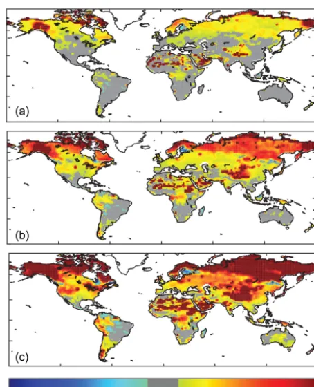
Next we consider whether using LAI adds information compared to precipitation, which is more traditionally used in climate change impacts assessments (e.g., Stocker et al., 2013; Field et al., 2014). General correlations between precipitation and LAI will be discussed in the next few sec-tions, but here we consider the spatial distribution of at-risk regions as defined by LAI or precipitation changes. To do this, we first consider the mean change in normalized precip-itation (Fig. 5a) and the % low precipprecip-itation (Fig. 5b), both defined equivalently to the LAI values (Sect. 2.2; Figs. 2c and 4c, respectively) for the model simulations considered here. Broadly speaking, the changes in precipitation seem to occur in similar regions as the changes in LAI, with large in-creases in precipitation over the high latitudes, and dein-creases over the subsidence zones of the tropics, as seen previously (e.g., Meehl et al., 2007; Tebaldi et al., 2011). Note that re-quiring the mean change to be statistically significant is a much stricter criteria than just an increase in low LAI, and thus the area identified in the two methods is quite differ-ent (Fig. 5a vs. Fig. 5b). Overlaying the regions from LAI and precipitation which are either one standard deviation
be-low the mean on average in the models (Fig. 5c) or see an increase in % Low values (Fig. 5d) suggests that LAI and precipitation largely show similar areas being at risk due to climate change, but there are significant regions which do not overlap. This suggests that there is potentially additional in-formation for climate impact studies using LAI projections rather than using precipitation alone (Fig. 5c, d). One of the most noticeable differences between LAI and precipitation projections is in the Mediterranean region where precipita-tion is projected to decrease, but LAI is not. Conversely, LAI projections suggest that some parts of South America and southern Africa are likely to experience more stress, which are not identified using precipitation. Future studies should consider whether the results of the LAI projections are use-ful for impact studies specifically in these regions.
3.3 Drivers of LAI projections
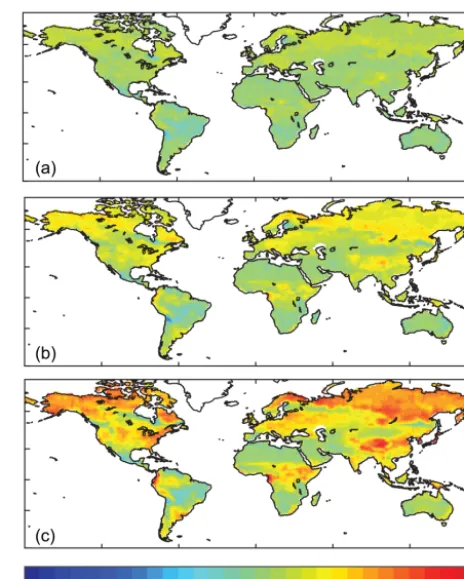
Figure 4.Mean of the models for the fraction of the time during which the annual mean LAI is considered “Low” (model projected annual mean LAI is less than 1 standard deviation of the current mean at each gridbox) is shown for 2011–2030 (a), 2041–2060 (b) and 2081–2100 (c) for RCP85, where the current mean and stan-dard deviation are defined for each grid box for 1981–2000. For the current climate, the fraction of time below 1 standard deviation will be 0.16, which is colored in gray, so all colors represent an increase in low LAI.
as simulated in the models to the model projections. Note that there are many other potential drivers of the projected LAI changes that are likely to be important, and thus our study only seeks to consider the most obvious interactions, and highlights the uncertainties in the model-specific drivers of LAI projections.
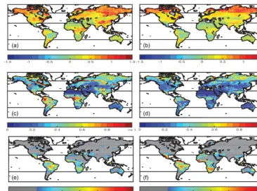
By correlating temperature and LAI projections at each grid box for each model we can look for potentially causal relationships between model projections of temperature and LAI (Fig. 6). This is analogous to using a ranked correla-tion coefficient to summarize the scatter in RCP8.5 points in Fig. 3, but at each grid box instead of the regional average. There are strong positive correlations between model simu-lated changes in temperature and LAI in some regions, es-pecially in parts of the northern high latitudes (Fig. 6a), sug-gesting that models with a projected larger warming in the high latitudes also simulate larger increases in LAI. Higher temperatures may drive higher LAI, however it is important to recall that correlation does not necessary imply
causa-tion. For example, higher LAIs could also be driving higher temperatures through LAI influence on surface albedo and changing surface energy fluxes (e.g., Lawrence and Slingo, 2004; Kala et al., 2014). In contrast to high latitudes, there are strong negative correlations across most of the tropics and subtropics (Fig. 6a).
The projected changes in precipitation are strongly corre-lated with projected changes in LAI across different models in many locations (Fig. 6b). This is consistent with the model mean analysis (Sect. 3.2) that showed that for most locations changes in LAI occur in the same locations as changes in precipitation (Fig. 5). The correlations seen in this analysis for RCP 8.5 are similar for the RCP4.5 (Fig. S6).
Next, we examine the correlation across models between the modeled changes in vegetation carbon stocks and change in LAI between current conditions and 2081–2100 (Fig. 6c). The relationship between LAI and vegetation carbon is not straightforward, and depends on the specific biophysics and biogeochemistry algorithms used in the models. Many ESMs calculate photosynthetic rates per unit leaf area; these rates are then extrapolated to canopy-level gross primary produc-tion using LAI and other variables (e.g., light, nitrogen and CO2availability and leaf physiological parameters) (e.g., see Bonan et al., 2011; Piao et al., 2008). The simulated in-creases in LAI are correlated across models with simulated increases in plant carbon stocks in many low-LAI regions, including many deserts, grasslands, and tundra ecosystems (Fig. 6c). Leaves compose most or all of the aboveground plant biomass in these ecosystems (e.g., Friedlingstein et al., 1999), such that increases in LAI relate directly to in-creases in plant carbon stocks. Changes in LAI correlate more poorly with simulated changes in plant carbon stocks in other regions, with small or negative correlations in many boreal, temperate, and tropical forested regions (Fig. 6c). Leaves typically compose only 3–5 % of aboveground plant biomass in forests (Friedlingstein et al., 1999), and closed-canopy forests can contain widely variable stocks of woody biomass that typically depend more on successional status than LAI or growth rate. Differences in the fractional com-position and turnover of these leaf- and woody tissues should decouple changes in LAI from changes in carbon stocks in woody biomass. As an example, in the CLM (the land model for the CESM-BGC) CO2fertilization causes a larger increase to wood allocation (62 %) than to leaf allocation (21 %) in the Southeastern US (D. Lombardozzi, personal communication, 2015). Thus, the issue of how LAI responds in different models is interesting and should be considered in future studies.
Figure 5.Mean of all models for the change in annual mean precipitation for 2081–2100 compared to current (1981–2000), normalized by the model standard deviation for RCP8.5 (similar to Fig. 2c, but for precipitation) (a). Mean of the models percent of the time during which the annual mean precipitation is 1 standard deviation below current values (similar to (c), but for precipitation) for 2081–2100 in RCP8.5 (b). Grid-boxes identified as statistically significantly decreasing in LAI (green) or precipitation (blue) or both (red) (i.e., the blue regions in Figs. 2a and 6a contrasted) (c). Grid-boxes identified as having an increase in the amount of time with low LAI (green) or precipitation (blue) or both (red) (i.e., the blue regions in Figs. 5c and 6b contrasted) (c).
we might expect models that respond more strongly with increased carbon uptake under higher CO2 conditions (i.e., largerβ land) to have greater vegetation carbon and LAI in the future. Globally the correlation with β land is 0.46 for vegetation carbon and−0.21 for LAI, suggesting that while some of the differences in future vegetation carbon projec-tions across models are due to differences in the model sim-ulation of CO2fertilization, LAI changes are not necessarily related to CO2 fertilization. At a regional extent there are interesting differences. For tropical, mid-latitude and high-latitude regions, respectively, theβ-land correlation for veg-etation carbon is 0.29, 0.47 and 0.60, and forβland and LAI these values are−0.18,−0.09 and 0.21. Thus for high lat-itudes, especially, the projections of LAI appear to be de-pendent on the way the models’ simulate the carbon dioxide fertilization.
It should be noted that it is difficult to identify from the correlations whether relationships are due to modeled CO2 fertilization effect or modeled simulation of LAI in the cur-rent climate. There are only two models with a low carbon dioxide fertilization effect (CESM-BGC and NOR-ESM). For high latitudes both models simulate low LAI for present day and small increases to future LAI. Thus either, or both factors could be important. These similarities likely come from both models using the same land carbon model (Thorn-ton et al., 2009) which includes nitrogen limitation. In the tropics the carbon dioxide fertilization is negatively corre-lated to future LAI changes, and only slightly correcorre-lated with vegetation carbon. The negative correlation in the tropics be-tween LAI projections and CO2 fertilization could be due to the smaller temperature impact on carbon cycle (γ land
Figure 7.Mean of all models for the annual mean change in LAI over time (2081–2100) relative to current (1981–2000), normalized by each model’s current (1981–2000) standard deviation at each grid point (a) for all models (same as Fig. 1c) and (b) for the top models, defined as the models performing in the top half (Table 4) for each region, tropical, mid-latitude or high-latitude. Because different models are included in different regions, there can be discontinuities at the boundaries in Fig. 8b (e.g., 30 and 60◦latitude). The standard deviation in the mean future projection at 2081–2100 across the models at each grid point are shown for (c) all models and (d) top models. Indication of “Low” LAI is the model mean fraction of the time that LAI is more than 1 standard deviation below the current mean LAI and is shown for (e) all models (same as Fig. 5c) and (f), top models for the period 2081–2100, where the current mean and standard deviation are defined for each grid box for 1981–2000. For the current climate, the fraction of the time below 1 standard deviation will be 0.16, which is colored in gray, so all colors represent an increase in drought.
from Arora et al., 2013) in the nitrogen-limited models (i.e., the β land andγ land are negatively correlated in Table 2 of Arora et al., 2013). These models see a strong increase in nitrogen mineralization in the tropics in a warming climate, which allows an increase in productivity in the future tropics (Thornton et al., 2009). Across these simulations, whether or not the model includes dynamic vegetation does not signifi-cantly correlate with changes in LAI in any of the regions.
Overall, the relationship of land model characteristics and LAI is not straightforward, which argues that more analy-sis of the complicated interactions between the details of the land biophysics and biogeochemistry, as well as biogeogra-phy changes is required in order to better understand and im-prove model projections of LAI.
4 The relationship between model skill and future projections
There are large differences between the different models’ projections of future LAI (e.g., Figs. 3, S5, 7b). Previous studies have hypothesized that they could reduce the
(a) Mean model/obs (b) Seasonal stddev model/obs (c) IAV stddev model/obs 4
3
2
1
0
4
3
2
1
0
4
3
2
1
0
Global Trop Mid High Global Trop Mid High Global Trop Mid High
(d) Annual mean spatial corr. (e) Avg. Seas. Corr.
1.0 0.8
0.6
0.4
0.2
0.0
1.0 0.8
0.6
0.4
0.2
0.0
Global Trop Mid High Global Trop Mid High
1.0
0.5
0.0
-0.5
-1.0
Global Trop Mid High (f) LAI vs. T Avg Corr
* * * *
1.0
0.5
0.0
-0.5
-1.0
Global Trop Mid High (g) LAI vs. time Avg Corr.
* * * *
Figure 8.Comparison of model metrics for the LAI comparisons from Table 2 across the models, for each region (global, tropical, mid-latitude and high mid-latitude) for (a) mean of the model divided by mean of the observations, (b) seasonal SD mean of the model divided by mean of the observations, (c) IAV SD mean of the model divided by mean of the observations, (d) spatial correlation of model to observed LAI, (e) average temporal correlation for seasonal variability, (f) average IAV LAI correlation with temperature (∗indicates observed value), (g) average IAV LAI correlation with time (∗indicates observed value).
advantages and disadvantages of using this type of approach are discussed in more detail in Flato et al. (2013). Here we do not advocate that such an approach leads to a better projec-tion, but rather simply use this approach to characterize the future model projections.
4.1 Evaluation of model LAI
Several recent studies have evaluated the land models in ESMs using the LAI satellite records (e.g., Anav et al., 2013a, b; Mao et al., 2013; Sitch et al., 2015). Thus we do not repeat those assessments, but rather briefly summarize the results of the comparisons here.
Most models tend to overestimate the mean LAI compared to the observations (Fig. 8a), and this is true at all latitudes (Fig. 8a, Table S2 in the Supplement). Several models have large overestimates (>50 % too high), including bcc-csm1,
bcc-csm1-1, BNU-ESM, GFDL-ESM2G, GFDL-ESM2M, MIROC-ESM. The over-prediction relative to the satellite data tend to be larger in tropical regions for most models, but the GFDL model estimates are also larger in the high lati-tudes (Fig. 8a, Table S2). However, the satellite-derived LAIs have biases; for example, they underestimate high LAIs due to being unable to see all the leaf layers in closed canopies or with high frequency of cloud cover or overestimate LAIs in more arid regions, and thus there may also be an error in the observational data set (see discussion in Vrieling et al., 2013; Anav et al., 2013b; Jong et al., 2013; Pfeifer et al., 2014 or Forkel et al., 2013, 2015, for example).
re-ME
V
ME
V
Models Models
Models Models
(a) Global (b) Tropical
(c) Mid-latitude (d) High-latitude
+
*Mean annualAnnual corr.
Seasonal SD Seasonal corr. IAV SD
Figure 9.Comparison of model metrics for the annual mean and seasonal metrics from Table 2 across the models for (a) global, (b) tropical, (c) mid-latitude and (d) high-latitude regions. Simi-lar information is shown in Tables S1 and S2, but here converted to the model evaluation value (Eq. 1) so that 1 is a perfect model simulation and lower values indicate worse simulations. Models are shown in Table 1, and listed in the figure. Metrics are mean annual (+), spatial correlation of mean annual (∗), seasonal cycle standard deviation(diamond), mean seasonal cycle correlation (triangle) and interannual variability (IAV) standard deviation (square).
gion in which they over-predict the strength of the seasonal cycle differs between models. Of course, there is not a strong seasonal cycle in the tropics, where the lowest standard de-viations tend to occur (Fig. 8e; Table S2a). Again, because of the difficulties of retrieving accurate LAI from satellites in closed canopies, the observations may underestimate the seasonal cycle in tropical forests.
Interannual variability tends to be over-predicted in some of the models (e.g., bcc-csm1, bcc-csm1_1, BNU-ESM, CESM1-BGC, GFDL-ESM2G, GFDL-ESM2M, MIROC-ESM, MIROC-ESM_CHEM) (Fig. 8c, Table S1). For this calculation, the interannual variability (IAV) is calculated as the standard deviation of the annual average across multi-ple years. Generally, the models do a decent job simulating the spatial variability in the annual mean LAI (Fig. 8d; Ta-ble S1), with the correlations being strongest in the tropics, and weakest in the high latitudes (Fig. 8d; Table S2). This is likely partly due to the strength of the LAI differences in tropics and the limitation of LAI primarily by moisture
alone (with low LAI in arid regions and high LAI in tropical forests). The timing of the seasonal cycle (Fig. 8e; Table S1) is less well simulated in the models, with several models not having an average statistically significant correlation (∼0.5 for 95 % significance for a 12-month seasonal cycle) on the global scale, or in the mid- and high latitudes (e.g., GFDL, ESM-MR on global scale, GFDL, inmcm4 and MPI-ESM-MR for various regions).
Next we explore the observed and modeled relationship between LAI and temperature, and the observed and modeled trend in LAI (e.g., Anav et al., 2013a, b; Ichii et al., 2002; Zeng et al., 2013; Mao et al., 2013; Zhu et al., 2013). As previously shown, there are positive relationships between modeled and measured LAI and temperature in high lati-tudes (Figs. 6a, S5; e.g., Anav et al., 2013a; Ichii et al., 2002; Zeng et al., 2013; Zhu et al., 2013). In the tropics (<30◦), the relationship can be positive or negative but some regions tend towards a negative relationship (Figs. S5, 6a). This is consistent with our understanding that many places in the tropics are close to the optimal growing temperature already, and increases may lead to reduced productivity (Lobell et al., 2011), although this also could be related to moisture stress (Fung et al., 2005). Compared to the observed cor-relations, most models have too strong of a negative rela-tionship between LAI and temperature in the tropics, and too strong of a positive relationship in the high latitudes (Fig. 8f, Table S2a–c). In the tropics, the BNU-ESM model has a weakly positive impact of temperature, while in the high lati-tudes, especially the CanESM2, CC, HadGEM2-ES, MPI-ESM-MR models have a much stronger correlation than observed. The model and observations show similarly weak correlations between the temperature and LAI in the mid-latitudes.
Some regions show substantial trends over time (1981– 2010) in measured LAI (Fig. S7b), especially in high lati-tudes in the Northern Hemisphere (e.g., Zhu et al., 2013; Mao et al., 2013). This could be associated with the longer grow-ing season due to warmgrow-ing (e.g., Lucht et al., 2002; Zeng et al., 2013). It is also possible that this trend is due to CO2 fer-tilization effects (e.g., Friedlingstein and Prentice, 2010). For high latitudes, we find a rank correlation of 0.58 across the models between the CO2fertilization factor on land for the earth system models (called theβland in Arora et al., 2013, as discussed above) and the average correlation of observed LAI with time, suggesting that there may be a component of carbon dioxide fertilization in the models’ temporal trends. These trends are stronger in the models than the observations, which may be related to an overestimate of the fertilization effect.
consid-ered could also lead to aliasing of the real variability, espe-cially in regions like the Sahel that have strong decadal scale variations (e.g., Loew, 2014). The observational data sets also contain measurement noise, while the model values do not. We expect the measurement noise to reduce the correlations of LAI with the environmental variables in the observations relative to the true values, as seen compared to many mod-els (Fig. 8f). Thus, our metrics for interannual variability are likely to be more impacted by uncertainty in the observations than for the annual mean or seasonal cycle, and thus they may be less useful for evaluation of the models, although potentially interesting. For this study, we consider the IAV in the annual mean, but there may be important changes in the seasonal cycle or length of growing season on an inter-annual time basis, which our simple approach does not con-sider (e.g., Murray-Tortarolo et al., 2013). In addition, the re-gional or global average of some of these correlations may be difficult to interpret, as it is not statistically significant (e.g., Fig. 8f), thus making the LAI IAV correlations less helpful.
Figure 9 summarizes our comparisons of the models with the observations for LAI for the different metrics in Table 2 (Tables S1, S2). In order to show both correlations and model mean biases in the same figure, we have converted the model-data comparisons into model evaluation values using Eq. (1) in Sect. 2.4, where 1 is a perfect model simulation and lower values represent worse model simulations. Overall, none of the models does a perfect job, and improving simulation of LAI for all models will be important. In addition, as dis-cussed above, some models perform better in some regions than others. In order to more easily see how the models com-pare, we also show the ranking of the different models in each region (Table 3). For this comparison, we exclude the magnitude and correlations in the IAV, because the observa-tional estimates for this are more likely to be in error than for the annual mean and seasonal analysis, as discussed above. Thus our overall evaluation of LAI in the models includes the following metrics: annual mean LAI, spatial correlation of annual mean, standard deviation of seasonal cycle and tem-poral correlation of the seasonal cycle. In the tropics the top three models are the INMCM4, the IPSL-CM5A-LR and the IPSL-CM5B-LR. For the mid-latitudes the top models are the CanESM2, IPSL-CM5A-MR and the HADGEM2-ES. For high-latitudes the top models are the BNU-ESM, bcc-csm1 and the MIROC-ESM_CHEM (Table 3; Fig. 9).
4.2 Future projections constrained by current model performance
Across broad regions, we evaluate which metrics are the most useful for potentially constraining future climate projections by considering how the metric is correlated with the projec-tions (Figs. 8, 9; Tables S1, S2). We consider four regions: the globe, tropics (latitudes<30◦), mid-latitudes (latitudes between 30 and 60◦), and high latitudes (latitudes>60◦). For the first approach, we look for the metrics that have the
high-Table 3.Model ranking based on performance on mean annual and seasonal cycle metrics for each region (see description in Sect. 2.1).
Tropical Mid-latitude High latitude
bcc-csm1 10 10 2
bcc-csm1-1 9 8 11
BNU-ESM 18 18 1
CanESM2 17 1 16
CESM1-BGC 6 11 17
GFDL-ESM2G 14 15 17
GFDL-ESM2M 16 17 6
HadGEM2-CC 10 5 7
HadGEM2-ES 14 3 11
inmcm4 1 8 13
IPSL-CM5A-LR 2 5 13
IPSL-CM5A-MR 4 1 9
IPSL-CM5B-LR 3 4 5
MIROC-ESM 12 15 4
MIROC-ESM_CHEM 13 14 2
MPI-ESM-LR 5 7 9
MPI-ESM-MR 7 12 15
NorESM1-ME 8 13 7
est correlation coefficient to constrain the future estimate of change in LAI (similar to Cox et al., 2013) (Fig. 10a, b). Us-ing this approach, we look for the model metrics (from Ta-ble 2) which have the highest correlations with future projec-tions across the models, for each of the regions. If we choose the models which do the best job with the metrics, this re-duces the number of models included in the projections, and may reduce model spread in projections.
As an example, for the globe, there are two metrics that correlate the highest with future projections: the average cor-relation of IAV in LAI with date (i.e., the trend), and the global mean LAI ratio of model to observation. This anal-ysis suggests that models with the largest relative change in LAI over the last 30 years (1980–2010) will have the largest change in LAI in the future (Fig. 10a). It also suggests that models with higher LAI in the current climate will have a larger change in the future (Fig. 10b). In Fig. 10a and b, the observation-based estimates are indicated by the gray vertical bar. Notice that the projected change in LAI given by mod-els that match best with the observations differs for different metrics, and thus it does not allow us to uniquely constrain the future projections (although it does suggest that the high-est values are the least likely). There is one model with a very large change in LAI in the future (BNU-ESM). We use Spearman rank correlations instead of Pearson correlations, so that these results are largely insensitive to the removal of one model.
(a) (b)
(c) (d) (e)
(g)
LAI IAV corr with date LAI mean model/obs
LAI IAV corr with date LAI mean model/obs Δ Precip (mm/day)
(f)
Seasonal Corr.
(h)
IAV (model/obs) Seasonal (model/obs)
Δ
LAI (m m )
2
–2
Δ
LAI (m /m )
2
2
A B C D E F G H I J K L M N O P Q R 1.2
0 0.4 0.8
0 0.2 0.4
1.2
0.4 0.8
0
1 2
Δ
LAI (m m )
2
–2
Δ
LAI (m m )
2
–2
Δ
LAI (m m )
2
–2
Figure 10.Scatterplot of the metrics with the highest absolute value of the correlation between the metric and future LAI changes across the globe (LAI IAV correlated with date (a) and mean LAI model/obs (b) tropics (<30◦) (LAI IAV correlated with date (c) and mean LAI model/obs d), mid-latitudes (between 30◦and 50◦) projected change in precipitation (e) and high-latitudes (>50◦) seasonal cycle average correlation (f), strength of IAV model/obs (g), and seasonal cycle strength model/obs (h). The symbols are in the shown colors for each model. The gray represents the value an ideal model would have based on the observations. The black line is the line that results from a linear regression of thexandyaxis.
high LAIs in the current climate and/or currently have large trends with time, tend to project higher LAI changes in the future. Again, these two metrics would constrain our future projections to two different LAI values, as the gray lines in-tersect with the slope at different LAI changes (Fig. 10c, d). For mid-latitudes, the highest correlation (and only statisti-cally significant correlation) is between the model predicted change in precipitation and LAI (Fig. 10e). Thus mid-latitude projections of LAI are difficult to constrain based on model metrics, but are sensitive to modeled changes in precipita-tion (as seen also in Fig. 5). For high latitudes there are three metrics with similar correlation coefficients: the average
tem-poral correlation in the seasonal cycle, the size of the inter-annual variability and the size of the seasonal cycle in LAI (Fig. 10f, g, h). Unfortunately again, these three metrics sug-gest a different projected change in LAI when the observed value is used to identify the models that are most realistic (gray line in Fig. 10f, g and h).
The second approach for characterizing the relationship between model simulations in the current climate and fu-ture climate projections, and potentially for reducing spread in the future projections follows the ideas of Steinacher et al. (2010). Here for each region, we chose the models that performed the best for several metrics (i.e., using the rank-ings in Table 3), instead of just one metric at a time (as above). For this study, we chose to use the top half of the models, based on their performance for each region (Table 3), so we include nine models out of the available 18 models for each region. Using this approach does change the mean future projections, especially for the tropics and high lati-tudes (Table 4; Fig. 7a vs. b), and does reduce the spread in the model values in the tropical region, but does not reduce the mean spread in mid-latitudes or high latitudes (Table 4; Fig. 7c vs. d). In the tropics, the top models tend to have lower future projections of changes in LAI than the average of all the models (0.07 m2m−2instead of 0.16 m2m−2). This is actually consistent with the analysis in Figure 10, since the models with the higher skill (close to gray line) would tend to have lower or middle values of future LAI projec-tions (Fig. 10a, b). For the mid-latitudes, there is not as much difference between using all models or the top performing models (Table 6), while for high latitudes, the top models tend to project slightly higher LAI in the future, also con-sistent with Fig. 10 f, g, h, where the projections from the models with more consistency with the observations tend to suggest higher LAI projections compared to including all the models.
The spatial distribution of the change in the future pro-jections using all models in comparison to the top models is consistent with the mean over the regions, with the largest change being seen across the tropics, with a reduction in both the mean LAI projection (Fig. 7a vs. b) as well as the stan-dard deviation (Fig. 7c vs. d). The changes from subsampling only the top performing models are not very large in most lo-cations in the mid- and high latitudes (Fig. 7a vs. b). Only in the tropics is the spread in the models reduced in the fu-ture projections (Fig. 7c vs. d). The fraction of the time that is considered to have low LAI in the future is increased in the tropics, if we only consider the top models compared to including all models (Fig. 7e vs. f).
Our results suggest that the better performing models tend to project lower LAIs in the future in the tropics in contrast to Cox et al. (2013), which focused on carbon–temperature relationships in the Amazon and which showed that obser-vational constraints on the models tend to suggest less loss in carbon under higher temperatures. However these results may not be inconsistent as they consider different metrics in different regions, and LAI is not necessarily linearly related to vegetative carbon or carbon uptake in the models (see dis-cussion in Sect. 3.4), suggesting that more analysis of how allocation is parameterized in the land carbon models is war-ranted.
Table 4.Mean and standard deviation across models for future pro-jections (LAI change in m2m−2) (2081–2100) for all models and for the top half of the models.
Tropics Mid-latitude High-latitude
Mean change
(all models) 0.16 0.35 0.31
(top models) 0.07 0.31 0.37
Standard deviation across models
(all models) 0.35 0.23 0.20
(top models) 0.25 0.24 0.24
Our analysis suggests that using multiple metrics does pro-vide information that allows us in some cases (especially the tropics) to change our mean future projection, and potentially reduce the spread between model predictions. Overall, in-cluding only the top models in the tropics projects a future with a smaller increase in mean LAI and an expansion in the regions at risk for a low LAI compared to including all mod-els. At high latitudes, focusing on the top models tends to increase the already large increase in mean in LAI compared to including all models.
5 Summary and conclusions
LAI is an important term for scaling leaf-level biogeophysi-cal and biogeochemibiogeophysi-cal processes to regional and global ar-eas, and thus it is vital to consider its change in future pro-jections. Here for the first time we consider LAI projections across the CMIP5 models and find that over much of the globe in the future, the models project an increase in mean LAI in the RCP8.5 scenario over the 21st century. Decreases are projected in the limited regions where there is also a projected decrease in mean precipitation; these regions are constrained primarily to the tropics. The change in LAI ap-pears to grow with carbon dioxide and temperature increases across regions over the 21st century (Fig. 3). Changes in LAI projected in the RCP4.5 are largely consistent with changes in RCP8.5, but have a reduced amplitude due to the smaller carbon dioxide and climate forcing.
For assessing climate change impacts, we propose that both mean LAI and LAI variability are important in iden-tifying vulnerable regions in future projections. The models project an increased frequency of low LAI conditions despite higher mean LAIs, especially in the tropics (Fig. 4). While much of the variability in LAI is driven by changes in pre-cipitation, projections of lower mean LAI or Low-LAI fquency can identify a slightly different set of vulnerable re-gions (Fig. 5), and add to the information that precipitation projections provide.
cli-mate to reduce the spread in the future projections (e.g., Flato et al., 2013), we conducted a brief comparison of the mod-els to available satellite-derived LAI data (Zhu et al., 2013), similar to previous analyses (e.g., Anav et al., 2013a, b; Mao et al., 2013; Sitch et al., 2015). Our results support the previ-ous conclusions that the modeled LAI could be improved in many aspects of the mean, seasonal and interannual variabil-ity, although difficulties in the observational data may pre-clude definitive assessment (Fig. 8).
We use two different methods for relating current model skill to model projections, and find that combining multiple metrics to choose better models (e.g similar to Steinacher et al., 2010) seems to work more robustly than simply cor-relating one metric against future projections (e.g., Cox et al., 2013; Hoffman et al., 2014), because the different met-rics suggest different future projections (Fig. 10). Overall, the top-performing models (top half of the models from Ta-ble 4) suggest smaller future increases in LAI in the tropics, and more regions with more incidences of low-LAI condi-tions than assessments that include all the models. This ap-proach also reduces the spread among models in the tropics. However, using only the top models did not make a large dif-ference in projections in the mid- and high latitudes (Fig. 7). Please note, however, that it is not clear that the models that perform best in the current climate have more accurate pro-jections, as discussed in more detail in Flato et al. (2013).
Finally, the spread among the models’ projections of LAI was correlated with the models’ projections of precipitation (Figs. 6b, 5). Thus our projections of LAI ultimately rest on the ability of models to project future precipitation. Unfortu-nately, in many regions the projected changes in precipitation are not large enough to be statistically significantly outside natural variability (e.g., Tebaldi et al., 2011) and there are discrepancies between climate model and statistical model predictions (e.g., Funk et al., 2014 vs. Tebaldi et al., 2011). In addition to precipitation affecting the future projections of LAI, increasing temperatures are likely to stress systems, even if there is additional rainfall (e.g., Lobell et al., 2011), expanding the regions at risk to increased drought (Fig. 5). Because of the importance of LAI for biophysical and bio-geochemical interactions, as well as the potential for LAI to be useful to the impacts community, we encourage more analysis of the drivers of LAI variability and changes in the future, as well as improvements in the model mechanisms responsible for the simulation of LAI.
The Supplement related to this article is available online at doi:10.5194/esd-7-211-2016-supplement.
Acknowledgements. We acknowledge the World Climate Research Programme’s Working Group on Coupled Modelling, which is responsible for CMIP, and we thank the climate modeling
groups (listed in Table 1 of this paper) for producing and making available their model output. For CMIP the U.S. Department of Energy’s Program for Climate Model Diagnosis and Intercom-parison provides coordinating support and led development of software infrastructure in partnership with the Global Organization for Earth System Science Portals. We acknowledge NSF-0832782 and 1049033 and assistance from C. Barrett and S. Schlunegger and the anonymous reviewers. We acknowledge the assistance of the LAI development group for making the LAI 3g product available, and the NOAA/OAR/ESRL PSD group for making the GPCP and GHCN gridded products available online at http://www.esrl.noaa.gov/psd/. This work was made possible, in part, by support provided by the US Agency for International Development (USAID) Agreement No. LAG-A-00-96-90016-00 through Broadening Access and Strengthening Input Market Systems Collaborative Research Support Program (BASIS AMA CRSP). All views, interpretations, recommendations, and con-clusions expressed in this paper are those of the authors and not necessarily those of the supporting or cooperating institutions.
Edited by: L. Ganzeveld
References
Anav, A., Murray-Tortarolo, G., Friedlingstein, P., Stich, S., Piao, S., and Zhu, Z.: Evaluation of Land Surface Models in Repro-ducing Satellite Derived Leaf Area Index over the High Latitude-Northern Hemisphere. Part II: Earth System Models, Remote Sensing, 5, 3637–3661, 2013a.
Anav, A., Friedlingstein, P., Kidston, M., Bopp, L., Ciais, P., Cox, P., Jones, C., Jung, M., Myneni, R., and Zhu, Z.: Evaluating the land and ocean components of the global carbon cycle in the CMIP5 earth system models, J. Climate, 26, 6801–6843, 2013b Arora, V. K., Scinocca, J., Boer, G. J., Christian, J., Denman, K. L.,
Flato, G., Kharin, V., Lee, W., and Merryfield, W.: Carbon emis-sion limits required to satisfy future representative concentration pathways of greenhouse gases, Geophys. Res. Lett., 38, L05805, doi:10.1029/2010GL046270, 2011.
Arora, V. K., Boer, G. J., Friedlingstein, P., Eby, M., Jones, C., Christian, J., Bonan, G., Bopp, L., Brovkin, V., Cadule, P., Ha-jima, T., Ilyina, T., Lindsay, K., Tjiputra, J. F., and Wu, T.: Carbon-Concentration and carbon-climate feedbacks in CMIP5 earth system models, J. Climate, 26, 5289–5314, 2013. Bentsen, M., Bethke, I., Debernard, J. B., Iversen, T., Kirkevåg,
A., Seland, Ø., Drange, H., Roelandt, C., Seierstad, I. A., Hoose, C., and Kristjánsson, J. E.: The Norwegian Earth Sys-tem Model, NorESM1-M – Part 1: Description and basic evalu-ation of the physical climate, Geosci. Model Dev., 6, 687–720, doi:10.5194/gmd-6-687-2013, 2013.
Bonan, G., Lawrence, P., Oleson, K., Levis, S., Jung, M., Reich-stein, M., Lawrence, D., and Swenson, S.: Improving canopy processes in the Community Land Model version 4 (CLM4) us-ing global flux fields empirically inferred from FLUXNET data, J. Geophys. Res., 116, G02014, doi:10.1029/2010JG001593, 2011.
Brown, M. and Funk, C.: Food security under climate change, Sci-ence, 319, 580–581, 2008.
Collins, W. J., Bellouin, N., Doutriaux-Boucher, M., Gedney, N., Halloran, P., Hinton, T., Hughes, J., Jones, C. D., Joshi, M., Lid-dicoat, S., Martin, G., O’Connor, F., Rae, J., Senior, C., Sitch, S., Totterdell, I., Wiltshire, A., and Woodward, S.: Develop-ment and evaluation of an Earth-System model – HadGEM2, Geosci. Model Dev., 4, 1051–1075, doi:10.5194/gmd-4-1051-2011, 2011.
Cook, K. and Vizy, E.: Coupled model simulations of the West African Monsoon System: Twentieth- and Twenty-First-Century Simulations, J. Climate, 19, 3681–3703, 2006.
Cox, P., Pearson, D., Booth, B., Friedlingstein, P., Huntingford, C., Jones, C., and Luke, C.: Sensitivity of tropical carbon to climate change constrained by carbon dioxide variability, Nature, 494, 341–344, 2013.
Cramer, W., Kicklighter, D. W., Bondeau, A., Iii, B. M., Churkina, G., Nemry, B., Ruimy, A., Schloss, A. L. and Intercomparison, ThE. P. OF. ThE. P. NpP. M. : Comparing global models of ter-rresrial net primary production (NPP): overview and key results, Glob. Change Biol., 5, 1–15, 1999.
Dufresne, J.-L., Foujols, M.-A., Denvil, S., et al.: Climate change projections using the IPSL-CM5 Earth system modl: From CMIP3 to CMIP5, Clim. Dynam., 40, 2123–2165, 2013. Dunne, J., John, J., Sheviliakova, E., Stouffer, R. J., Krasting, J.,
Malyshev, S., Milly, P., Sentman, L., Adcroft, A., Cooke, W., Dunne, K., Harrison, M., Krasting, J., Malyshev, S., Milly, P., Phillips, P., Sentman, L., Samuels, B., Spelman, M., Winton, M., Wittenberg, A., and Zadeh, N.: GFDL’s ESM2 global cupoled climate-carbon Earth system models. Part II: Carbon System for-mation and baseline simulation characteristics, J. Climate, 26, 2247-2267, 2013.
Fan, Y. and van den Dool, H.: A global monthly land surface air temperature analysis for 1948–present, J. Geophys. Res., 113, D01103, doi:10.1029/2007JD008470, 2008.
Field, C. B., Behrenfeld, M. J., Randerson, J. T., and Falkowski, P.: Primary Production of the Biosphere: Integrating Ter-restrial and Oceanic Components. Science, 281, 237–240 doi:10.1126/science.281.5374.237, 1998.
Field, C. B., Barros, V. R., Mach, K. J., et al.: Technical Summary, in: Climate Change 2014: Impacts, Adaptation, and Vulnerabil-ity. Part A: Global and Sectoral Aspects. Contribution of Work-ing Group II to the Fifth Assessment Report of the Intergovern-mental Panel on Climate Change, edited by: Field, C. B., Bar-ros, V. R., Dokken, D. J., Mach, K. J., Mastrandrea, M. D., Bilir, T. E., Chatterjee, M., Ebi, K. L., Estrada, Y. O., Genova, R. C., Girma, B., Kissel, E. S., Levy, A. N., MacCracken, S., Mastran-drea, P. R., and White, L. L., Cambridge University Press, Cam-bridge, United Kingdom and New York, NY, USA, 35–94, 2014. Flato, G., Marotzke, J., Abiodun, B., Braconnot, P., Chou, S. C., Collins, W., Cox, P., Driouech, F., Emori, S., Eyring, V., Forest, C., Gleckler, P., Guilyardi, E., Jakob, C., Kattsov, V., Reason, C., and Rummukainen, M.: Evaluation of Climate Models, in: Cli-mate Change 2013: The Physical Science Basis. Contribution of Working Group I to the Fifth Assessment Report of the Intergov-ernmental Panel on Climate Change, edited by: Stocker, T. F., Qin, D., Plattner, G.-K., Tignor, M., Allen, S. K., Boschung, J., Nauels, A., Xia, Y., Bex, V., and Midgley, P. M., Cambridge
Uni-versity Press, Cambridge, United Kingdom and New York, NY, USA, 2013.
Forkel, M., Carvalhais, N., Verbesselt, J., Mahecha, M., Neigh, C., and Reichstein, M.: Trend Change Detection in NDVI Time Se-ries: Effects of Inter-annual Variability and Methodology, Re-mote Sensing, 5, 2113–2144, doi:10.3390/rs5052113, 2013. Forkel, M., Migliavacca, M., Thonicke, K., Reichstein, M.,
Schaphoff, S., Weber, U., Carvalhais, N., 2015. Codominant wa-ter control on global inwa-terannual variability and trends in land surface phenology and greennes. Glob. Change Biol., 21, 3414– 3435, doi:10.1111/gcb.12950, 2015.
Friedlingstein, P., Joel, G., Field, C. B., and Fung, I. Y.: Toward an allocation scheme for global terrestrial carbon models, Glob. Change Biol., 5, 755–770, 1999.
Friedlingstein, P., Cox, P., Betts, R., Bopp, L., von Bloh, W., Brovkin, V., Cadule, P., Doney, S., Eby, M., Fung, I., Bala, G., John, J., Jones, C., Joos, F., Kato, T., Kawamiya, M., Knorr, W., Lindsay, K., Mathews, H. D., Raddatz, T., Rayner, P., Re-ick, C., Roeckner, E., Schnitzler, K.-G., Schnurr, R., Strassmen, K., Weaver, A. J., Yoshikawa, C., and Zeng, N.: Climate–carbon cycle feedback analysis, results from the C4MIP Model inter-comparison, J. Climate, 19, 3337–3353, 2006.
Friedlingstein, P., Meinshausen, M., Arora, V. K., Jones, A., Anav, A., Liddicoat, S., and Knutti, R.: Uncertainties in CMIP5 climate projections due to carbon cycle feedbacks, J. Climate, 27, 511– 526, doi:10.1175/JCLI-D-12-00579.1, 2013.
Friedlingstein, P. and Prentice, I. C.: Carbon-climate feedbacks: a review of model and observation based estimates, Current Opin-ion in Environmental Sustainability, 2, 251–257, 2010.
Fung, I., Doney, S., Lindsay, K., and John, J.: Evolution of car-bon sinks in a changing climate, P. Natl. Acad. Sci. USA, 102, 11201–11206, 2005.
Funk, C. and Brown, M.: Intra-seasonal NDVI change projections in semi-arid Africa, Remote Sens. Environ., 101, 249–256, 2006. Funk, C., Hoell, A., Shukla, S., Bladé, I., Liebmann, B., Roberts, J. B., Robertson, F. R., and Husak, G.: Predicting East African spring droughts using Pacific and Indian Ocean sea surface temperature indices, Hydrol. Earth Syst. Sci., 18, 4965–4978, doi:10.5194/hess-18-4965-2014, 2014.
Ganzeveld, L., Lelieveld, J., and Roelofs, G.-J.: A dry deposition parameterization for sulfur oxides in a chemistry and general cir-culation model, J. Geophys. Res., 103, 5679–5694, 1998. Gleckler, P., Taylor, K. E., and Doutriaux, C.: Performance
metrics for climate models, J. Geophys. Res., 113, D06104, doi:10.1029/2007JD008972, 2008.
Groten, S.: NDVI-crop monitoring and early yield assessment of Burkino Faso, Int. J. Remote Sens., 14, 1495–1515, 1993. Harris, I., Jones, P., Osborn, T., and Lister, D.: Updated
high-resolution grids of monthly climatic obsevations – the CRU TS3.10 dataset, Int. J. Climatol., 34, 623–642, doi:10.1002/joc.3711, 2013.
Hoffman, F., Randerson, J., Arora, V. K., Bao, Q., Cadule, P., Ji, D., Jones, C., Kawamiya, M., Khatiwala, S., Lindsay, K., Obata, A., Sheviliakova, E., Six, K., Tjiputra, J. F., Volodin, E., and Wu, T.: Causes and implications of persistent atmospheric carbon diox-ide biases in Earth System Models, J. Geophys. Res.-Biogeo., 119, 141–162, doi:10.1002/2013JG002381, 2014.