www.ocean-sci.net/13/303/2017/ doi:10.5194/os-13-303-2017
© Author(s) 2017. CC Attribution 3.0 License.
Technical note: Evaluation of three machine learning models
for surface ocean CO
2
mapping
Jiye Zeng1, Tsuneo Matsunaga1, Nobuko Saigusa1, Tomoko Shirai1, Shin-ichiro Nakaoka1, and Zheng-Hong Tan2 1Centre for Global Environmental Research, National Institute for Environmental Studies, Tsukuba, Ibaraki, Japan 2Institute of Tropical Agriculture and Forestry, Hainan University, Haikou, Hainan, China
Correspondence to:Jiye Zeng ([email protected])
Received: 6 September 2016 – Discussion started: 25 October 2016
Revised: 16 March 2017 – Accepted: 24 March 2017 – Published: 19 April 2017
Abstract. Reconstructing surface ocean CO2 from scarce measurements plays an important role in estimating oceanic CO2uptake. There are varying degrees of differences among the 14 models included in the Surface Ocean CO2Mapping (SOCOM) inter-comparison initiative, in which five models used neural networks. This investigation evaluates two neural networks used in SOCOM, self-organizing maps and feed-forward neural networks, and introduces a machine learning model called a support vector machine for ocean CO2 map-ping. The technique note provides a practical guide to select-ing the models.
1 Introduction
The global ocean is a major sink for anthropogenic carbon and therefore an important contributor to slowing down the human-induced global warming (Stocker et al., 2013). To calculate the oceanic CO2uptake, various models have been used to interpolate scarce CO2measurements in the surface ocean spatially and temporarily to obtain basin-wide (e.g., Zeng et al., 2002; Lefèvre et al., 2005; Chierici et al., 2006; Sarma et al., 2006; Jamet et al., 2007; Friedrich and Oschlies, 2009; Telszewski et al., 2009; Takamura et al., 2010; Land-schützer et al., 2013; Nakaoka et al., 2013; Iida et al., 2015; Goddijn-Murphy et al, 2015) and global ocean CO2 maps (Takahashi et al., 2002, 2009, 2014; Park et al., 2010; Rö-denbeck et al., 2013; Sasse et al., 2013; Jones et al., 2015; Zeng et al., 2015). The Surface Ocean CO2 Mapping (SO-COM) inter-comparison initiative revealed varying degrees of differences among 14 models (Rödenbeck et al., 2015), of which 5 used neural networks. They include self-organizing
maps (SOMs) and feedforward neural networks (FNNs). The SOM has a long history in CO2 mapping (Lefèvre et al., 2005; Friedrich and Oschlies, 2009; Telszewski et al., 2009; Nakaoka et al., 2013). Recently, the FNN has been gaining popularity in this field (Landschützer et al., 2015; Zeng et al., 2014, 2015). In this investigation we introduce a machine learning model called a support vector machine (SVM) for ocean CO2 mapping and compare the SVM with the SOM and FNN. We intend to provide a practical guide for using these machine learning models.
2 Model equations
The machine learning models included in this study cannot directly model the long-term trend of CO2. Therefore, we ex-press the dependence of CO2fugacity (fCO2)on year (YR), month (MON), latitude (LAT), and longitude (LON) as the sum of a nonlinear static component and a linear trend com-ponent:
fCO2=Fstatic(LAT,LON,MON)+Ftrend(YR). (1) As available observations are scarce with respect to the biogeochemical properties of the surface ocean, we used sea surface temperature (SST), sea surface salinity (SSS), chlorophyll-a concentration (CHL), and mixed layer depth (MLD) as the proxy variables of space and time. These proxy variables were commonly used by models included in the SOCOM. The model equation becomes
They have a circular property and therefore cannot be used directly. For instance, longitude −180◦ is geographically
connected to longitude 180◦, but numerically they appear
to be two extreme longitude values to the models. Zeng et al. (2014, 2015) circumvented this problem by using sine and cosine transformed components. Their approach could unintentionally enhance the influence of LON and MON on fCO2as one more derived variable from each of them was added to the model. We excluded LON in the belief that the combination of SST, SSS, CHL, and MLD contains sufficient spatial information, but retained LAT for its different sea-sonal and geophysical meanings in the Northern and South-ern hemispheres. Replacing MON with dSST also improves the expression of the effect of season geographically.
3 Data
We extracted monthlyfCO2from the track-gridded database of the Surface Ocean CO2 Atlas (SOCAT) version 3.01 (Pfeil et al., 2013; Sabine et al., 2013; Bakker et al., 2014). The database has a 1◦×1◦ spatial resolution and includes global measurements from 1970 to 2014. Similar to Zeng et al. (2014), we excluded some data points by these crite-ria: (i) fCO2 values smaller than 250 µatm or larger than 550 µatm, (ii) ocean depth smaller than 500 m, (iii) salin-ity smaller than 25.0, and (iv) year before 1990. A total of 158 052 data points were extracted with these conditions.
The monthly SST data of 1990 to 2015 were extracted from the Optimum Interpolation (OI) V2 product2of NOAA (Reynolds et al., 2002). The monthly SSS climatology was extracted from the World Ocean Atlas 2013 (WOA13) prod-uct3(Boyer et al., 2013), which contains the monthly mean SSS from 27 June 1896 to 25 December 2012. The monthly CHL climatology was calculated using the MODIS Aqua and SeaWiFS climatology4, which covers the period of 2012 to 2015. The mean of the two CHLs was used as the CHL clima-tology. The mixed layer data were derived from the Monthly Isopycnal and Mixed-layer Ocean Climatology5 of NOAA (Schmidtko et al., 2013), which includes the period of 1955 to 2012.
4 Machine learning models
The Appendix and Table 1 summarize the algorithms of the three models. Here we focus on discussing their usage in CO2mapping.
1http://www.socat.info/
2http://www.esrl.noaa.gov/psd/data/gridded/data.noaa.oisst.v2. html
3https://www.nodc.noaa.gov/OC5/woa13/ 4https://oceancolor.gsfc.nasa.gov/cgi/l3 5http://www.pmel.noaa.gov/mimoc/
The trend in Eq. (2) cannot be modeled directly by the models. One approach to dealing with the problem is to normalize the measurements to a reference year using a global rate and to only model the nonlinear component. Zeng et al. (2014) presented a method to model the linear compo-nent in Eq. (2). Instead of repeating the process, we used their annual rate of 1.5 µatm to remove the trend fromfCO2 to normalize it to the reference year 2005, i.e.,
fCOnormalized2 =fCO2−1.5·(YR-2005). (3) Although Takahashi et al. (2014) obtained a global mean rate of 1.9 µatm yr−1, we used 1.5 µatm yr−1as this rate was ob-tained by using the griddedfCO2of SOCAT version 2. The normalizedfCO2was used to model the nonlinear compo-nent in Eq. (2). In later discussions,fCO2means the nor-malizedfCO2unless explicitly stated. Similarly, we applied the log transform of Zeng et al. (2014) to CHL prior to data scaling discussed below, i.e.,
CHL=log10(1.0+CHL). (4)
4.1 SMV
For a given dataset, the SVM requires a prior step to find the optimal value for the parameterσ in Eq. (A10) and the parameterγ in Eq. (A11). To shorten the training time, we randomly chose 10 % of the measurement data in this step and obtained 0.06 forσ and 10 for γ. Note that these val-ues are dependent on data scaling, which is necessary in this case to avoid the overflow problem in solving Eq. (A18). We scaled all input variables LAT, SST, SSS, CHL, MLD, and dSST by their minimum and maximum to confine them in the range (0, 1), i.e.,
v= v−vmin
vmax−vmin. (5)
4.2 FNN
Data scaling is not necessary for the FNN, but can improve its performance. Following Zeng et al. (2014), we scaled the input variables by their mean and standard deviation as v=v−v
s . (6)
The output variablefCO2is scaled by v=0.1+0.8 v−vmin
vmax−vmin. (7) This confines the scaledfCO2to between 0.1 and 0.9 for better response to changes in input variables. The kernel function Eq. (A4) has the property that for any input in (−∞,
Table 1.Feature comparison of the three machine learning models.
Feature SVM FNN SOM
Input space projection Projects the input variable space to a high-dimensional space that is propor-tional to the number of training sam-ples.
Projects the input space to a high-dimensional space that is proportional to the number of hidden neurons and in-put variables.
Projects the input space to a feature space whose size is determined by the number of neurons.
Prediction by Continuous interpolation. Continuous interpolation. Picking up labeling samples that have the closest feature to the input.
Problems May over-fit and over-interpolate. May over-fit and over-interpolate. Discrete interpolation leads to spatial discontinuity.
Data scaling Helps in solving the linear equation, but has no effect on the result.
Helps the convergence of training, but has an insignificant effect on the result.
Significant effect on the result.
Results affected by The parameter values for regularization and kernel function.
The number of hidden neurons. The number of neurons and data scal-ing.
We used 64 hidden neurons for the FNN as Zeng et al. (2014) did. The learning rate in Eq. (A6) was set to 0.25 by trial-and-error. A small value makes training slow, whereas a large value may make a training diverge. The constant in Eq. (A8) was determined dynamically in each iterative train-ing loop. It was taken as 10 times the mean of absolute dif-ferences between modeled and observedfCO2. We experi-enced that this method improves the performance of training.
4.3 SOM
Data scaling is critical for the SOM, as the distance defined by Eq. (A1) would be affected by variable units. We used Eq. (6) to scale input variables in training the SOM. Based on our preliminary correlation analysis, we applied a factor of 2 to enhance the influence of SST and CHL on the distance. Using such a subjective factor is the only way to make the correlations between the output and the input variables more in line with observed correlations.
From the labeling procedure of SOM described in the Ap-pendix, it is not difficult to see that the number of neuron cells in SOM affects the labeling and hence the prediction. Unfor-tunately, there is no guideline for choosing the size. Based on previous studies (Telszewski et al., 2009; Nakaoka et al., 2013), we used 20 000 neuron cells, roughly one neuron cell for one 1×1 grid cell of sampled areas.
5 Model validation
We examined the goodness of fit by randomly selecting 10 to 50 % of the data points to train the FNN and SVM, and to label the SOM; and then calculated the correlation coef-ficient between modeled and observed CO2 of the selected data points.
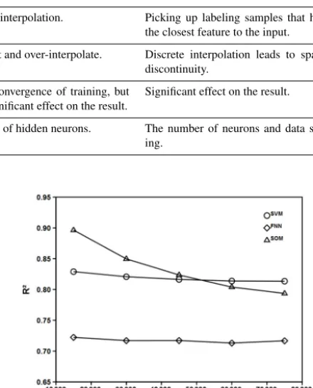
The SOM yields the best correlation in the case of 10 % of randomly selected data points and the correlation decreases with the number of data points (Fig. 1). The reason is that for
Figure 1.Correlation coefficient between modeled and observed
fCO2(uatm). The sample size is the number of data points ran-domly selected to train FFN and SVM and to label SOM.
a given number of neuron cells, the fewer the data points, the less likely a neuron cell will be labeled by multiple measure-ments and the more likely that the prediction will find the same CO2value used for labeling. Therefore, the goodness of fit does not necessary mean good SOM modeling.
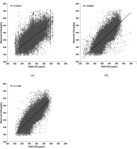
Figure 2.Predicted vs. observedfCO2(µatm). Ten percent of data points were selected randomly to train FNN and SVM and to label SOM, and the rest was used for validation.
whereas the latter is determined by the number of training data. For 6 input variables, 15 000 training data, and 64 hid-den neurons, the number of parameters is 509 for the FNN and 15001 for the SVM.
A better indicator of the performance of the models would be the goodness of prediction. To emulate the situation that the sampled area was only a small portion of the global ocean, we evaluated the goodness of prediction by train-ing FNN and SVM and labeltrain-ing SOM with 10 % of ran-domly selected data to make a prediction for the rest of the data. Figure 2 shows that the SVM yielded the best cor-relation (R2=0.72), the FNN fell behind (R2=0.67), and the SOM performed the worst (R2=0.54). The differences between predicted and observed fCO2 are 0.1±17.4 µatm for SVM, 0.1±18.9 µatm for FNN, and 0.2±23.3 µatm for SOM. Compared to the variation of fCO2 measurements, these differences are small and their uncertainties are on the same order of magnitude as the variation of measurements. Let us examine the standard deviation (SD) offCO2in those grids with at least three data points. The track-griddedfCO2 in SOCAT version 3.0 includes an SD ranging from 0.1 to 71.2 µatm and the mean is 5.2 µatm. Calculating the SD of normalizedfCO2in the same grids and in the same months of all years yielded a mean of 12.5 µatm in the range of 0.1 to 103.1 µatm. The normalization had little effect on the SD as the calculation for non-normalized fCO2gives a mean SD of 14.6 µatm in the range of 0.1 to 107.5 µatm.
From the algorithm of SOM in the Appendix, it is not dif-ficult to see that the SOM does not make extrapolation – the model always approximates new inputs by the measure-ments used for training and approximatesfCO2by the mea-surements used for labeling; therefore, the predictedfCO2 values are within the observedfCO2 range (Fig. 2a). Fig-ure 2c shows that the extrapolated fCO2 by the SVM, if any, did not exceed the observed range. To investigate the ex-trapolation risk, we used 200 000 data points randomly gen-erated for SST, dSST, SSS, MLD, and CHL in the range of (0, 40◦C), (−20, 20◦C), (20, 50), (1, 1500 m), and (0 log(mg m−3), 2 log(mg m−3)), respectively. These ranges are larger than the corresponding observed ranges of (0, 34◦C), (−13, 16◦C), (24, 40), (1, 1000 m), and (0 log(mg m−3), 1.2 log(mg m−3)). The SVM and FNN produced fCO2 in the range of (267, 468 µatm) and (199, 596 µatm), respectively, for the simulated samples. Compared to the observedfCO2 range of (240, 560 µatm), the experiment indicates that the over-extrapolation risk of the SVM is low.
6 Differences
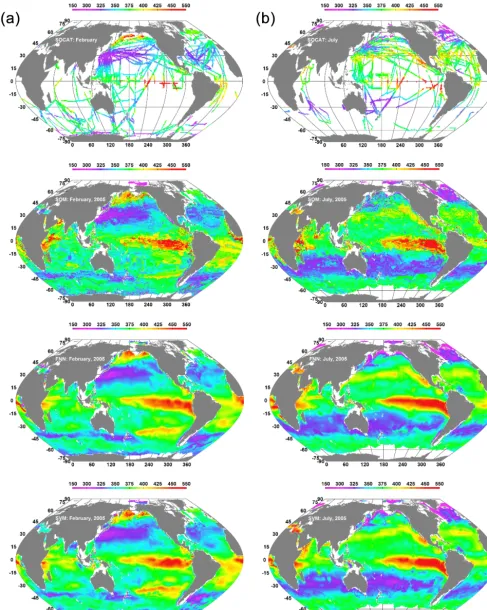
Figure 3 shows fCO2 maps in February and July 2005, which is the reference year for normalization. In the map-ping, we randomly selected 50 % of the data to train the FNN and SVM and to label the SOM. All models captured the major features of observedfCO2distribution. The SOM ex-hibits obvious discontinuity because of its discrete character-istics of picking upfCO2values from the labeled SOM. For year 2005, the meanfCO2difference is−0.05±12.73 µatm for FNN−SVM and−0.6±18.80 for SOM−SVM. The un-certainty is the standard deviation of the mean difference be-tween predicted and observed values. The statistics indicates that FNN agrees better with SVM than SOM does.
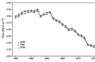
Figure 4.Modeled global CO2fluxes. A negative value indicates oceanic uptake.
On the spatial scale of tens of degrees, the three mod-els show good mutual agreement for modeled fCO2 dis-tributions among them. However, each model shows distin-guished fine structures, which are determined by the biogeo-chemical processes in the ocean, by model parameters ob-tained from training, and by the characteristics of the models. We believe that the modeled monthlyfCO2distributions are true to the degree given by the model validations.
7 Summary
The main features of the three machine models are listed in Table 1. The SVM is recommended when the computer has enough memory to store the matrix in Eq. (A18), which is proportional to the square of the number of training data. The SVM performs the best, but the training time could become very long when the number of training data is too large to be handled by a computer without using virtual memory. For any given dataset, using the SVM requires a prior step to find the optimal value for the parameter σ in Eq. (A10) and the parameterγ in Eq. (A11).
The FNN model does not perform as well as the SVM, but the number of training data does not affect its training as much as the SVM’s. The training time can become long when a large number of hidden neurons are used and many iterations are needed to achieve convergence. It takes a longer time to train the FNN than the SVM for a small number of data points. However, the FNN is simpler to use as it re-quires no prior step. However, it may have the risk of over-extrapolation.
The SOM is recommended only when the other two mod-els have over-fitting or over-interpolation problems. The SOM performs the worst and is not as straightforward as the others as its result depends too much on data scaling and the number of neurons. An advantage of the SOM is that once trained, re-labeling the SOM with new CO2 measurements and making a new prediction is fast. Although the SOM does not have the over-extrapolation problem of the FNN, it may produce nonsense predictions due to its strong dependence on data scaling.
In areas where there was no measurement on a large scale, predictions made by the models must be treated conser-vatively, as SVM and FNN may produce extrapolated re-sults and SOM may extract CO2from unexpected provinces. Figure 3 shows that the modeled CO2 east of the African coast near the Equator in July 2005 (Fig. 3) appeared much higher than the nearby measurements, which were made in July 1995 and adjusted to 2005 using the global rate of 1.5 µatm yr−1. However, considering the large variations of the rate from region to region (Takahashi et al., 2014) and of the repeated measurements discussed in Sect. 5, the mea-surements were not sufficient to support rejecting the mod-eled CO2. Similar CO2 hotspots occurred in the Southern Ocean west of South America in February 2005, around the latitudinal zone of 50◦S. The modeled CO2 distribu-tions by Takahashi et al. (2014) also showed CO2hotspots around the latitudinal zone of 30◦S in the same month and region. Their model used a completely different interpola-tion scheme based on a diffusion–advecinterpola-tion transport model for surface waters. In principle, this hotspot CO2 was pro-duced by our models using measurements somewhere else where the biogeochemical properties were similar to those in the hotspot areas. As the SOM does not make extrapolation, the SVM has a low possibility of over-extrapolation, and the hotspots appeared in all models, the risk of accepting them would not be high.
Data availability. The software and data used by this study are available at https://figshare.com/s/38488b7003b03e2103c9.
Appendix A: Self-organizing map
A self-organizing map (SOM) is a type of artificial neu-ral network that is trained using unsupervised learning (Ko-honen, 1984). The SOM in our application comprises grid points on a two-dimensional plane. Each grid point, also called a neuron cell, has the same number of parameters as the input variables, which include LAT, SST, SSS, CHL, MLD, and dSST in our case. Training the SOM is to use samples of input variables to adjust the parameters to make neighborhood neuron cells with similar parameter values that reflect certain biogeochemical features of the surface ocean.
We used the batch learning algorithm (Abe et al., 2002) to train the SOM as the result does not depend on the sequential order of training samples. The parameters were initialized randomly in the range (−1, 1). In each iterative training loop, each training sample is associated with a neuron cell to which the distance defined as follows is smaller than to other neuron cells:
d= |f(p−x)|, (A1) wherepdenotes the vector of neuron cell parameters,x the vector of input variables, andfthe scale matrix that we in-troduced to change the influence of certain variables on the distance. The components offare all 0 except for those on the diagonal, which are set to 1 by default. In our application, the data for each input variable were scaled to be unitless by its mean and standard deviation to eliminate the effect of units on the distance.
The associated neuron cell is called the best matching cell (BMC). After the BMCs for all training samples are found, the parameters are updated by
pi =
P
khikxk
P
khik
, (A2)
where i andk denote indexes of neuron cells and training samples, respectively. The neighborhood function that deter-mines the weight factorhis defined as
hik=exp(−
|rik|
q ), (A3)
where|rik|denotes the geographic distance between theith neuron cell and the BMC of thekth training sample andqis a factor that decreases linearly with the iteration loop. In other words, the procedure adjusts the parameters of neuron cells toward those training samples whose BMCs are close to them and the amount of adjustment decreases exponentially with the geographic distance between neuron cells and linearly with the training loop.
The trained SOM needs to be labeled byfCO2for making predictions. The values offCO2measurements are assigned to their BMC. PredictingfCO2for a set of input variables is realized by finding the BMC labeled withfCO2and extract-ing its meanfCO2value.
A1 Feedforward neural network
A feedforward neural network (FNN) is an artificial neural network that is trained using supervised learning. Our FNN comprises three layers (Zeng et al., 2014): an input layer, a hidden layer, and an output layer. The number of neurons in the input layers is determined by the number of input vari-ables, i.e., LAT, SST, SSS, CHL, MLD, and dSST in our case. The output layer has only one neuron forfCO2. Each neu-ron in the hidden layer uses the following kernel function to transform all input variables:
yh=
1
1+exp −(b+wTx), (A4)
wherewdenotes the vector of weight parameters andb the offset parameter. Theyhof all hidden neurons become the in-puts of the output neuron, which uses the same kernel func-tion to transformyhto producefCO2.
The training updates the offset and weight parameters, which are initialized randomly in the range (−1, 1), by min-imizing the cost function
f w0
=1
2e Te=1
2|ym−yo|
2, (A5)
wherew0is the extended vector that includes bandw; y
m andyostand for the vectors of modeled and observedfCO2, respectively. In the gradient descent training algorithm, up-datingw0at the training iterationtcan be expressed as
w0(t )=w0(t−1)−αg (A6) whereαis the learning rate (a positive number smaller than 1), andgthe first-order derivative of the cost function g= ∇f w0
=JTe, (A7)
whereJis the Jacobian matrix whose components are deriva-tives of e with respect to w0 using the back propagation method. We used the efficient Levenberg–Marquardt algo-rithm (Wilamowski et al., 2010), which derives the gradient as
g=JTJ+µI
−1
JTe, (A8)
whereµis a constant.
A2 Support vector machine
wherex stands for a set of measurements of the input vari-ables,cthe vector of coefficients,bthe offset parameter, and φthe kernel function. In this investigation, we used the radial basis kernel function, i.e.,
ϕ(xi)Tϕ xj=exp −
xi−xj
2
2σ2
!
, (A10)
whereσ is a parameter whose optimal value depends on the data used for training. The subscription ofxindicates a sam-ple of input variables.
Given a set of training samples {xk, yk}N
k=1, the goal of training SVM is to minimize the cost function
F (c)=1
2
cTc+γeTe (A11)
where
ek=yk−cTϕ (xk)−b (A12)
andγis a constant whose optimal value depends on the data used for training. The Lagrangian solution for the optimiza-tion problem of Eq. (A11) is given by
L (c, e, b, α)=1
2(c
Tc+γ|e|)
−XN
kαk
n
cTϕ (xk)+b+ek−yk
o
, (A13)
whereαkis a Lagrangian multiplier. The optimal conditions of Eq. (A13) are
∂L ∂ck
=0 →ck=αkϕ (xk) , (A14)
∂L
∂b =0 →
XN
kαk=0, (A15)
∂L ∂ek
=0 → αk=γ ek, (A16)
∂L ∂αk
=0,→ ckϕ (xk)+b+ek−yk=0. (A17) After eliminatingcandefrom the above conditions, the following equation is obtained:
0 uT
u +γ−1I b α
=
0 y
, (A18)
whereu is a vector with all components being 1, and the components ofare
ij =ϕ(xi)Tϕ xj. (A19)
Once Eq. (A18) is solved, making a prediction is done by y(x)=XN
kαkϕ(xk)
Competing interests. The authors declare that they have no conflict of interest.
Acknowledgements. The Surface Ocean CO2 Atlas (SOCAT) is an international effort, endorsed by the International Ocean Carbon Coordination Project (IOCCP), the Surface Ocean Lower Atmosphere Study (SOLAS), and the Integrated Marine Biogeo-chemistry and Ecosystem Research program (IMBER), to deliver a uniformly quality-controlled surface ocean CO2 database. The many researchers and funding agencies responsible for the collec-tion of data and quality control are thanked for their contribucollec-tions to SOCAT.
Edited by: J. M. Huthnance
Reviewed by: three anonymous referees
References
Abe, T., Kanaya, S., Kinouchi, M., Ichiba, Y., Kozuki, T., and Ike-mura, T.: A Novel Bioinformatic Strategy for Unveiling Hid-den Genome Signatures of Eukaryotes: Self-Organizing Map of Oligonucleotide Frequency, Genom. Inform., 13, 12–20, 2002. Bakker, D. C. E., Pfeil, B., Smith, K., Hankin, S., Olsen, A., Alin,
S. R., Cosca, C., Harasawa, S., Kozyr, A., Nojiri, Y., O’Brien, K. M., Schuster, U., Telszewski, M., Tilbrook, B., Wada, C., Akl, J., Barbero, L., Bates, N. R., Boutin, J., Bozec, Y., Cai, W.-J., Castle, R. D., Chavez, F. P., Chen, L., Chierici, M., Cur-rie, K., de Baar, H. J. W., Evans, W., Feely, R. A., Fransson, A., Gao, Z., Hales, B., Hardman-Mountford, N. J., Hoppema, M., Huang, W.-J., Hunt, C. W., Huss, B., Ichikawa, T., Johan-nessen, T., Jones, E. M., Jones, S. D., Jutterström, S., Kitidis, V., Körtzinger, A., Landschützer, P., Lauvset, S. K., Lefèvre, N., Manke, A. B., Mathis, J. T., Merlivat, L., Metzl, N., Murata, A., Newberger, T., Omar, A. M., Ono, T., Park, G.-H., Pater-son, K., Pierrot, D., Ríos, A. F., Sabine, C. L., Saito, S., Salis-bury, J., Sarma, V. V. S. S., Schlitzer, R., Sieger, R., Skjelvan, I., Steinhoff, T., Sullivan, K. F., Sun, H., Sutton, A. J., Suzuki, T., Sweeney, C., Takahashi, T., Tjiputra, J., Tsurushima, N., van Heuven, S. M. A. C., Vandemark, D., Vlahos, P., Wallace, D. W. R., Wanninkhof, R., and Watson, A. J.: An update to the Surface Ocean CO2Atlas (SOCAT version 2), Earth Syst. Sci. Data, 6, 69–90, doi:10.5194/essd-6-69-2014, 2014.
Basak, D., Pal, S., and Patranabis, D. C.: Support vector regression, Neu. Inf. Pro.-Letters and Reviews, 11, 203–224, 2007. Boyer, T. P., Antonov, J. I., Baranova, O. K., Coleman, C., Garcia,
H. E., Grodsky, A., Johnson, D. R., Locarnini, R. A., Mishonov, A. V., O’Brien, T. D., Paver, C. R., Reagan, J. R., Seidov, D., Smolyar, I. V., and Zweng, M. M.: World Ocean Database 2013, NOAA Atlas NESDIS 72, edited by: Levitus, S. and Mishonov, A., Technical Ed., Silver Spring, MD, 209 pp. 2013.
Chierici, M., Fransson, A., and Nojiri, Y.: Biogeochemical pro-cesses as drivers of surfacefCO2in contrasting provinces in the subarctic North Pacific Ocean, Global Biogeochem. Cy., 20, GB1009, doi:10.1029/2004GB002356, 2006.
Dee, D. P., Uppala, S. M., Simmons, A. J., Berrisford, P., Poli, P., Kobayashi, S., Andrae, U., Balmaseda, M. A., Balsamo, G., Bauer, P., Bechtold, P., Beljaars, A. C. M., van de Berg, L.,
Bid-lot, J., Bormann, N., Delsol, C., Dragani, R., Fuentes, M., Geer, A. J., Haimberger, L., Healy, S. B., Hersbach, H., Hólm, E. V., Isaksen, L., Kållberg, P., Köhler, M., Matricardi, M., McNally, A. P., Monge-Sanz, B. M., Morcrette, J.-J., Park, B.-K., Peubey, C., de Rosnay, P., Tavolato, C., Thépaut, J.-N., and Vitart, F.: The ERA-Interim reanalysis: configuration and performance of the data assimilation system, Q. J. Roy. Meteor. Soc., 137, 553–597, 2011.
Friedrich, T. and Oschlies, A.: Neural network-based esti-mates of North Atlantic surface pCO2 from satellite data: A methodological study, J. Geophys. Res., 114, C03020, doi:10.1029/2007JC004646, 2009.
Goddijn-Murphy, L. M., Woolf, D. K., Land, P. E., Shutler, J. D., and Donlon, C.: The OceanFlux Greenhouse Gases methodol-ogy for deriving a sea surface climatolmethodol-ogy of CO2 fugacity in support of air–sea gas flux studies, Ocean Sci., 11, 519–541, doi:10.5194/os-11-519-2015, 2015.
Iida, Y., Kojima, A., Takatani, Y., Nakano, T., Sugimoto, H., Mi-dorikawa, T., and Ishii, M.: Trends inpCO2and sea-air CO2 flux over the global open oceans for the last two decades, J. Oceanogr., 71, 637–661, 2015.
Jamet, C., Moulin, C., and Lefèvre, N.: Estimation of the oceanic
pCO2 in the North Atlantic from VOS lines in-situ measure-ments: parameters needed to generate seasonally mean maps, Ann. Geophys., 25, 2247–2257, doi:10.5194/angeo-25-2247-2007, 2007.
Jones, S. D., Quéré, C. L., Rödenbeck, C., Manning, A. C., and Olsen, A.: A statistical gap-filling method to interpolate global monthly surface ocean carbon dioxide data, J. Adv. Model. Earth Syst., 7, 1942–2466, 2015.
Kohonen, T.: Self-Organization and Associative Memory, Springer, Berlin, 1984.
Landschützer, P., Gruber, N., Bakker, D. C. E., Schuster, U., Nakaoka, S., Payne, M. R., Sasse, T. P., and Zeng, J.: A neu-ral network-based estimate of the seasonal to inter-annual vari-ability of the Atlantic Ocean carbon sink, Biogeosciences, 10, 7793–7815, doi:10.5194/bg-10-7793-2013, 2013.
Landschützer, P., Gruber, N., Haumann, F., Rödenbeck, C., Bakker, D., van Heuven, S., Hoppema, M., Metzl, N., Sweeney, C., Taka-hashi, T., Tilbrook, B., and Wanninkhof, R.: The reinvigoration of the Southern Ocean carbon sink, Science, 349, 1221–1224, 2015.
Lefèvre, N., Watson, A. J., and Watson, A. R.: A comparison of multiple regression and neural network techniques for mapping in situpCO2data, Tellus B, 57, 375–384, 2005.
Nakaoka, S., Telszewski, M., Nojiri, Y., Yasunaka, S., Miyazaki, C., Mukai, H., and Usui, N.: Estimating temporal and spatial varia-tion of ocean surfacepCO2in the North Pacific using a self-organizing map neural network technique, Biogeosciences, 10, 6093–6106, doi:10.5194/bg-10-6093-2013, 2013.
Park, G.-H., Wanninkhof, R., Doney, S. C., Takahashi, T., Lee, K., Feely, R. A., Sabine, C. L., Triñanes, J., and Lima, I. D.: Variability of global net sea-air CO2fluxes over the last three decades using empirical relationships, Tellus B, 62, 352–368, doi:10.1111/j.1600-0889.2010.00498.x, 2010.
Pelckmans, K., Suykens, J. A. K., Gestel, T. V., Brabanter, J. D., Hamers, B., Moor, D., and Vandewalle, J.: LS-SVMlab: a MATLAB/C toolbox for Least Squares Support Vector Ma-chines, http://www.esat.kuleuven.ac.be/sista/lssvmlab, last ac-cess: April 2017, presented at Neural Information Processing Systems (NIPS 2002), 2002.
Pfeil, B., Olsen, A., Bakker, D. C. E., Hankin, S., Koyuk, H., Kozyr, A., Malczyk, J., Manke, A., Metzl, N., Sabine, C. L., Akl, J., Alin, S. R., Bates, N., Bellerby, R. G. J., Borges, A., Boutin, J., Brown, P. J., Cai, W.-J., Chavez, F. P., Chen, A., Cosca, C., Fassbender, A. J., Feely, R. A., González-Dávila, M., Goyet, C., Hales, B., Hardman-Mountford, N., Heinze, C., Hood, M., Hoppema, M., Hunt, C. W., Hydes, D., Ishii, M., Johannessen, T., Jones, S. D., Key, R. M., Körtzinger, A., Landschützer, P., Lauvset, S. K., Lefèvre, N., Lenton, A., Lourantou, A., Merlivat, L., Midorikawa, T., Mintrop, L., Miyazaki, C., Murata, A., Naka-date, A., Nakano, Y., Nakaoka, S., Nojiri, Y., Omar, A. M., Padin, X. A., Park, G.-H., Paterson, K., Perez, F. F., Pierrot, D., Poisson, A., Ríos, A. F., Santana-Casiano, J. M., Salisbury, J., Sarma, V. V. S. S., Schlitzer, R., Schneider, B., Schuster, U., Sieger, R., Skjel-van, I., Steinhoff, T., Suzuki, T., Takahashi, T., Tedesco, K., Tel-szewski, M., Thomas, H., Tilbrook, B., Tjiputra, J., Vandemark, D., Veness, T., Wanninkhof, R., Watson, A. J., Weiss, R., Wong, C. S., and Yoshikawa-Inoue, H.: A uniform, quality controlled Surface Ocean CO2 Atlas (SOCAT), Earth Syst. Sci. Data, 5, 125–143, doi:10.5194/essd-5-125-2013, 2013.
Reynolds, R. W., Rayner, N. A., Smith, T. M., Stokes, D. C., and Wang, W.: An Improved In Situ and Satellite SST Analysis for Climate, J. Climate, 15, 1609–1625, 2002.
Rödenbeck, C., Keeling, R. F., Bakker, D. C. E., Metzl, N., Olsen, A., Sabine, C., and Heimann, M.: Global surface-ocean
pCO2 and sea–air CO2 flux variability from an observation-driven ocean mixed-layer scheme, Ocean Sci., 9, 193–216, doi:10.5194/os-9-193-2013, 2013.
Rödenbeck, C., Bakker, D. C. E., Gruber, N., Iida, Y., Jacobson, A. R., Jones, S., Landschützer, P., Metzl, N., Nakaoka, S., Olsen, A., Park, G.-H., Peylin, P., Rodgers, K. B., Sasse, T. P., Schus-ter, U., Shutler, J. D., Valsala, V., Wanninkhof, R., and Zeng, J.: Data-based estimates of the ocean carbon sink variability – first results of the Surface OceanpCO2Mapping intercompari-son (SOCOM), Biogeosciences, 12, 7251–7278, doi:10.5194/bg-12-7251-2015, 2015.
Sabine, C. L., Hankin, S., Koyuk, H., Bakker, D. C. E., Pfeil, B., Olsen, A., Metzl, N., Kozyr, A., Fassbender, A., Manke, A., Malczyk, J., Akl, J., Alin, S. R., Bellerby, R. G. J., Borges, A., Boutin, J., Brown, P. J., Cai, W.-J., Chavez, F. P., Chen,
A., Cosca, C., Feely, R. A., González-Dávila, M., Goyet, C., Hardman-Mountford, N., Heinze, C., Hoppema, M., Hunt, C. W., Hydes, D., Ishii, M., Johannessen, T., Key, R. M., Körtzinger, A., Landschützer, P., Lauvset, S. K., Lefèvre, N., Lenton, A., Lourantou, A., Merlivat, L., Midorikawa, T., Mintrop, L., Miyazaki, C., Murata, A., Nakadate, A., Nakano, Y., Nakaoka, S., Nojiri, Y., Omar, A. M., Padin, X. A., Park, G.-H., Pater-son, K., Perez, F. F., Pierrot, D., PoisPater-son, A., Ríos, A. F., Sal-isbury, J., Santana-Casiano, J. M., Sarma, V. V. S. S., Schlitzer, R., Schneider, B., Schuster, U., Sieger, R., Skjelvan, I., Stein-hoff, T., Suzuki, T., Takahashi, T., Tedesco, K., Telszewski, M., Thomas, H., Tilbrook, B., Vandemark, D., Veness, T., Watson, A. J., Weiss, R., Wong, C. S., and Yoshikawa-Inoue, H.: Surface Ocean CO2 Atlas (SOCAT) gridded data products, Earth Syst. Sci. Data, 5, 145–153, doi:10.5194/essd-5-145-2013, 2013. Sarma, V. V. S. S., Saino, T., Sasaoka, K., Nojiri, Y., Ono, T., Ishii,
M., Inoue, H. Y., and Matsumoto, K.: Basin-scalepCO2 distri-bution using satellite sea surface temperature, Chla, and climato-logical salinity in the North Pacific in spring and summer, Global Biogeochem. Cy., 20, GB3005, doi:10.1029/2005GB002594, 2006.
Sasse, T. P., McNeil, B. I., and Abramowitz, G.: A new constraint on global air-sea CO2fluxes using bottle carbon data, Geophys. Res. Lett., 40, 1594–1599, 2013.
Schmidtko, S., Johnson, G. C., and Lyman, J. M.: MI-MOC: A global monthly isopycnal upper-ocean climatol-ogy with mixed layers, J. Geophys. Res., 118, 1658–1672, doi:10.1002/jgrc.20122, 2013.
Stocker, T., Qin, D., and Platner, G.-K.: Climate Change 2013 The Physical Science Basis, Cambridge University Press, Cambridge, United Kingdom, 2013.
Takahashi, T., Sutherland, S. C., Sweeney, C., Poisson, A., Metzl, N., Tilbrook, B., Bates, N., Wanninkhof, R., Feely, R. A., Sabine, C., Olafsson, J., and Nojiri, Y.: Global sea-air CO2flux based on climatological surface oceanpCO2, and seasonal biological and temperature effects, Deep-Sea Res. Pt. II, 49, 1601–1622, 2002. Takahashi, T., Sutherland, S. C., Wanninkhof, R., Sweeney, C., Feely, R. A., Chipman, D. W., Hales, B., Friederich, G., Chavez, F., Sabine, C., Watson, A., Bakker, D. C. E., Schuster, U., Metzl, N., Yoshikawa-Inoue, H., Ishii, M., Midorikawa, T., Nojiri, Y., Körtzinger, A., Steinhoff, T., Hoppema, M., Olafsson, J., Arnar-son, T. S., Tilbrook, B., Johannessen, T., Olsen, A., Bellerby, R., and Wong, C. S.: Climatological mean and decadal change in surface oceanpCO2, and net sea-air CO2flux over the global oceans, Deep-Sea Res. Pt. II, 56, 554–577, 2009.
Takahashi, T., Sutherland, S. C., Chipman, D. W., Goddard, J. G., Ho, C., Newberger, T., Sweeney, C., and Munro, D. R.: Cli-matological distributions of pH,pCO2, total CO2, alkalinity, and CaCO3saturation in the global surface ocean, and temporal changes at selected locations, Mar. Chem., 164, 95–145, 2014. Takamura, T. R., Inoue, H. Y., Midorikawa, T., Ishii, M., and Nojiri,
Y.: Seasonal and Inter-Annual Variations inpCO2sea and Air-Sea CO2 Fluxes in Mid-Latitudes of the Western and Eastern North Pacific during 1999–2006: Recent Results Utilizing Vol-untary Observation Ships, J. Meteorol. Soc. Jpn., 88, 883–898, 2010.
Ríos, A. F., Steinhoff, T., Santana-Casiano, M., Wallace, D. W. R., and Wanninkhof, R.: Estimating the monthly pCO2 distri-bution in the North Atlantic using a self-organizing neural net-work, Biogeosciences, 6, 1405–1421, doi:10.5194/bg-6-1405-2009, 2009.
Wanninkhof, R., Park, G.-H., Takahashi, T., Sweeney, C., Feely, R., Nojiri, Y., Gruber, N., Doney, S. C., McKinley, G. A., Lenton, A., Le Quéré, C., Heinze, C., Schwinger, J., Graven, H., and Khatiwala, S.: Global ocean carbon uptake: magnitude, variabil-ity and trends, Biogeosciences, 10, 1983–2000, doi:10.5194/bg-10-1983-2013, 2013.
Wilamowski, B. M. and Yu, H.: Improved Computation for Levenberg-Marquardt Training, IEEE T. Neural Networ., 21, 930–937, 2010.
Zeng, J., Nojiri, Y., Landschützer, P., Telszewski, M., and Nakaoka, S.: A global surface oceanfCO2climatology based on a feed-forward neural network, J. Atmos. Ocean Tech., 31, 1838–1849, 2014.
Zeng, J., Nojiri, Y., Nakaoka, S., Nakajima, H., and Shirai, T.: Sur-face ocean CO2 in 1990-2011 modelled using a feed-forward neural network, Geoscience Data Journal, 2, 47–51, 2015. Zeng, J. Y., Nojiri, Y., Murphy, P. P., Wong, C. S., and Fujinuma,