Based on Generalized Type-II Progressive Hybrid Censoring Scheme
S.K. Ashour
Department of Mathematical Statistics
Institute of Statistical Studies & Research, Cairo University, Egypt [email protected]
A. Elshahhat
Department of Accounting& Quantitative Information Systems Faculty of Technology & Development, Zagazig University, Egypt [email protected]
Abstract
Bayesian and non-Bayesian estimators are obtained for the unknown parameters of Weibull distribution based on the generalized Type-II progressive hybrid censoring scheme and different special cases are obtained. The asymptotic variance covariance matrix and approximate confidence intervals based on the asymptotic normality of the maximum likelihood estimators are obtained. Bayes estimates and Bayes risks have been developed under a squared error loss function using informative and non-informative priors for the unknown Weibull parameters. It is observed that the estimators obtained are not available in closed forms, although they can be easily evaluated for a given sample by using suitable numerical methods. Therefore, a numerical example is considered to illustrate the proposed estimators.
Keywords: Asymptotic Variance Covariance Matrix; Bayes Estimator; Bayes Risk; Generalized Type-II Progressive Hybrid Censoring Scheme; Maximum Likelihood Estimator; Weibull Distribution.
1. Introduction
In reliability studies and life-testing experiments, the failure time data of experimental items are often not completely available. Reducing the cost and time associated with the experiments is crucial in statistical experiments with censored data. Kundu and Joarder (2006) proposed a progressive hybrid censoring scheme (PHCS). This scheme has become quite popular in reliability and lifetime testing studies. Childs et al. (2008) proposed Type-II PHCS for the purpose of increasing the efficiency of statistical analysis as well as saving the total test time. The drawback of the Type-II PHCS is that far fewer than m failures may be observed and it might take a very long time to observe m-th
failures and complete the life test. For this motivation, Lee et al. (2015) proposed a generalized Type-II PHCS, which the experiment is guaranteed to terminate at a pre-fixed time.
estimation for the unknown parameters of Weibull distribution under the generalized Type-II PHCS and special cases are given. The asymptotic variance covariance matrix and the approximate confidence interval based on the asymptotic normality of the
maximum likelihood estimators (MLEs) are obtained. In Section 4, the Bayes estimates and the Bayes risks under squared error loss (SEL) function for the Weibull parameters based on generalized Type-II PHCS are provided. In Section 5, a numerical example is considered to illustrate the proposed estimators. The paper finally ends with a brief conclusion given in Section 6.
2. Model Description
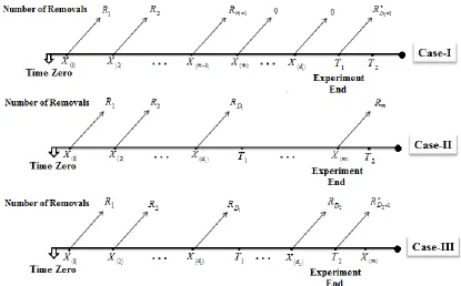
Generalized Type-II PHCS proposed by Lee et al. (2015), to overcome the drawbacks of Type-II PHCS. This censoring scheme can be described as follows: Consider a life test in which n identical items are put on test. Assume that X 1 ,X 2 ,...,X n denote the corresponding lifetimes from a distribution with the cumulative distribution function
(CDF), F x
, and the probability density function (PDF), f x
. The integer m, times1
T and T2 are pre-assigned such that mn and 0 T1 T2 , and also R R1, 2,...,Rm
are pre-assigned integers satisfying
1
m i
i R m n
. Let D1 and D2denote the numberof observed failures up to time T1 and T2, respectively. Similarly, the number of survival units withdrawn at times T1 and T2 are
1
1 *
1 1 1
m
D i i
R n d
R and2 2
*
1 2 1
d
D i i
R n d
R , respectively.The experiment terminated at time T*max
T1, min
X m ,T2
, all of the remaining units at the terminated time T* are withdrawn from the experiment. If X m T1, then instead of terminating the test by withdrawing the remaining Rm items after the m-thfailure, the researcher continue to observe failures but without any further withdrawals up to time T1, therefore,
1
1 0
m m D
R R R . If T1X m T2, terminate the test at m
Figure 1: Schematic illustration of generalized Type-II PHCS
Based on the generalized Type-II PHCS, the observed data will be one of the following three forms:
1
1
2
1 2
1 1
1 2
1
1 2 1
Case-I : ,..., , ,..., , if , Case-II : ,..., ,..., , if , Case-III : ,..., ,..., , if .
m m d m
d m m
d m m
X X X X X T T
X X X T X T
X X X T T X
and, the likelihood function for this censoring scheme is given by
* 1
1 1
* 2
1 2
1 1 1 1 2
2 1 1 2
3 2 1 2
1
; 1 ; 1 , if ,
; 1 ; , if , (1)
; 1 ; 1 , if .
j D
j
j D
D R R
j j m
j
R m
j j m
j
D R R
j j m
j
f x F x F T X T T
L X f x F x T X T
f x F x F T T T X
where,
1
1
1 1 ,
m D
k j
k j
R
2 1
1 ,
m m
k j
k j
R
2
3
1 1 ,
m D
k j
k j
R
1
1 *
1 1 1
m
D i i
R n d
R and 2 2*
1 2 1
d
D i i
3. Maximum Likelihood Estimation
The Weibull distribution has been extensively used to model lifetimes and material strengths. Johnson et al. (1994) presented a detailed account of this distribution and its
properties. Suppose that the observed failure times are independent identically distributed (iid) Weibull distribution with PDF
1; , x , 0, , 0.
f x xe x (2) and CDF is
; ,
1 x , 0, , 0.F x e x (3) where and are the shape and scale parameters, respectively. The Rayleigh distribution is a special case of the two-parameter Weibull distribution when the shape parameter 2 and is a suitable model for life testing studies. Suppose the lifetime random variable X has a Rayleigh distribution with PDF
2; 2 x , 0, 0.
f x xe x
(4)
and CDF is
2; 1 x ,
0, 0.
F x e x
(5)
where is a scale parameter.
Based on the PDF and the CDF of Weibull distribution (2) and (3), respectively, the likelihood function of the generalized Type-II PHCS (1), then
1 *1 1 11
2 *
2 2 21
1 1 1 1 1 1 2 1 1 1 3 1 1 2 1 2 1 2 ,
, (6)
, if
, , if
, if .
j j D j j j j D D x R
D T R
j m
j
m x R
m
j m
j
D
x R
D T R
j m
j
x e e
x e
x e e
X T T
L X T X T
T T X
where,
1
1
1 1 ,
m D k j k j R
2 1
1 ,
m m k j k j R
2 31 1 ,
m D k j k j R
1 1 *1 1 1
m
D i i
R n d
R and 2 2*
1 2 1
d
D i i
R n d
R . The likelihood functions (6) can be combined and rewritten as:
1 1
1 1 , , i i Si j i j j S S j j
x R W
x e L X
(7)where i 1, 2,3;
1 1,
S D
1
* 1 1 D 1
2 ,
S m W2
0, for Case-II, and3 2,
S D
2
* 3 2 D 1
W T R ,
for Case-III.
The corresponding log likelihood function of (7) can be written as
1 1, log 1 log
1 ,
i
i
S
i j j
S
j i
j j
l X S x
x R W
(8)Differentiating (8) with respect to and , we get
1 1
ln
log 1 log log ,
i i
S S
i
j i q
j j j
j j
S L
x x R x W T
and
1 ln 1 . i S i j i j j S Lx R W
(9)Equating the first derivations (9) to zero and solving for ˆ and ˆ, we get the MLE ˆ andˆ of and , respectively, in the following forms
ˆ
1 ˆ ˆ , ˆ 1 i i ii i S
j i i
j j
S
x R W
(10) and
ˆ
1 1 ˆ ˆ = ,ˆ ˆ i i 1 log ˆ log i
i
i i S S
i i j j j j i i q j j
S
x R x W T x
(11)where i 1, 2,3 and q 1, 2 for i 1,3, respectively.
The Fisher information matrix
I
,
is then obtained by taking the negative expectation for the second partial derivatives from the natural logarithm likelihood function (8). Since this expectation is difficult to obtained, so, under some regularity conditions, ( , ) ˆ ˆ is approximately bivariately normal with mean
,
and the asymptotic variance covariance matrixI
01
,
. Practically,I
01
,
can be estimate byI
01( , ) ˆ ˆ , then
1 2 2 2 10 2 2
2
ˆ ˆ,
ln ln ˆ
ˆ ˆ
Var Cov ,
ˆ
ˆ, ,
ˆ ˆ
ln ln Cov , Varˆ
I
L L
where the elements of the observed information matrix are as follows:
2 2
2
2 2 1
ln
1 log log ,
i
S i
j i q
j j
j
S L
x R x W T
2
1
ln
1 log log
i
S
j i q
j j
j
L
x R x W T
,and
2
2 2
lnL Si
Clearly, the MLEs can be obtained by solving set of nonlinear equations, this needs computer facilities and numerical technique.
Now, we propose a confidence intervals for the unknown Weibull parameters and under generalized Type-II PHCS based on the asymptotic distribution of the MLEs ˆ and ˆ (10) and (11), respectively, then 100 1
% approximate confidence intervals for and can be obtained using the asymptotic normality of the MLEs ˆ and ˆ as follows
2
ˆ z . Var ˆ
and ˆz2. Var
ˆ ,where Var
ˆ and Var
ˆ are the first and the second elements on the main diagonal of the asymptotic variance covariance matrix (12), respectively, and z2 is the upper2 -th
percentile of a standard normal distribution.
Lee et al. (2015) results in the case of exponential distribution can be obtained as a special case from above results by putting 1 and replacing by 1 . We get to corresponding new results based on Rayleigh distribution as a special case, i.e., for 2 and using the PDF and the CDF of Rayleigh distribution (4) and (5), respectively, then the MLEs will be the solution of the following log likelihood function:
log 1log 1 2
1
,i i
S S
i j j j j j i
l X S
x
x R W (13)where i 1, 2,3;
1 1,
S D
1
2 * 1 1 D 1
W T R , for Case-I,
2 ,
S m
W2 0, for Case-II,
and
3 2,
S D
2
2 * 3 2 D 1
Equating the first derivations from (13) to zero and solving forˆ, the MLE ˆ of taken the following form
2
1
ˆ , 1, 2,3.
1 i
i
i S
j i
j j
S
i
x R W
Again, computer facilities and numerical techniques must be used to solve this set of nonlinear equations.
4. Bayesian Estimation
Bayes estimators and the corresponding Bayes risks using SEL function under the assumption of gamma prior distributions of the unknown parameters of the Weibull distribution will be obtained based on generalized Type-II PHCS. We consider Bayesian estimation under the assumption that and are independently distributed with gamma prior distributions. Assumed that ~Gamma c d
, and ~Gamma a b
, . Therefore, the joint prior density of and can be written with proportional as follows
1 1 , , , 0
, c a e d b , a b c d
(14)
For the non-informative priorsa b c d 0, the joint prior density (14) becomes
,
1
.Based on the likelihood function (7) and the joint prior density (14), the joint posterior density of and given the data x can be written with proportional as follows
, x
,
.L
, x
,
hence,
1
1 1 1
1 1
. ,
Si
j j
j i
i i
x R
d W b
S c S a
C V e
x e
(15)
where i 1, 2,3;
1
i
j
S
j
V x
,
1 1,
S D
1
* 1 1 D 1
W T R , for Case-I,
2 ,
S m W2
0, for Case-II, and3 2,
S D
2
* 3 2 D 1
W T R , for Case-III,
the normalizing constant C1 in (15) is given by
1 1
1
0 0
1 1
. Si
j j
j i
i i x R W b d
S c S a
C V e d d
The normalizing constant C1 can be obtained using computer facilities and numerical techniques. Using the non-informative priors a b c d 0, the posterior distribution (15) can be rewritten with proportional as follows:
1
1 1 1 . , S i j j j i i i
x R W
S S V x e
From (15), we can obtain the marginal distributions of and , respectively, as follows:
The marginal PDF of is given by
,
,f x x d
1 1, 0 .
1 i i i d i S a S j i j j S c
V e S a
f x
x R W b
(16)The normalizing constant C2 in (16) is given by
2 0 1 1 1 i i i d i S a S j i j j S cV e S a
C d
x R W b
Similarly, the marginal PDF of will be
,
,f x x d
1 1 0
1 1
, 0 .
Si
j j
j i
i i
x R W b d
S c S a
f x V e d
(17)The normalizing constant C3 in (17) is given by
1 1
3 0 0
1 1 Si j j j i i i
x R W b d
S c S a
C V
e
d d
.Clearly, the marginal PDF of can be obtained in a closed form but the marginal PDF of (17) may be obtained by using the computer facilities and numerical techniques.
The SEL function
,
2will be used to obtain the Bayes estimator and the Bayes risk, respectively. Using (16) and (17) to obtain the Bayes estimators and for and under the SEL function as follows:
0 0 0 0
,
, , X ,
, X
U d d
where U
,
is the Bayes estimator for any function of and , that is
1 2 0
1
.
1 i
i
i d
i
S a
S
j i
j j
S c
V e S a
E X C d
x R W b
and
1 1 1 3 0 0
1
.
Si
j j
j i
i i
x R W b d
S c S a
E X C V e d d
Using the marginal PDF of and (16) and (17), respectively, the Bayes risk associated with and under the SEL function can be obtained as follows:
The Bayes risk associated with is given by
22
,
R E X E X
where,
2 1
2 0
1
1
1 i
i
i d
i
S a
S
j i
j j
S c
V e S a
E X C d
x R W b
.Similarly, the Bayes risk associated with is given by
22
,
R E X E X
where,
2
1 1 1 3 0 0
1 1
.
Si
j j
j i
i i
x R W b d
S c S a
E X C V e d d
Clearly, the Bayes estimate and the Bayes risk of and can be obtained using computer facilities and numerical techniques.
5. A Numerical Illustration
The performance of the results obtained in Sections 3 and 4 can't be compared theoretically, to illustrate the behavior of the proposed methods as well as evaluate the statistical performances of these estimates a numerical illustration is conducted. We shall use the real data set originally presented by Linhart and Zucchini (1986). The following data set is the failure times of the air conditioning system of an airplane. This data set was analyzed by Gupta and Kundu (2001). The ordered data with n 30 are as follows: 1, 3, 5, 7, 11, 11, 11, 12, 14, 14, 14, 16, 16, 20, 21, 23, 42, 47, 52, 62, 71, 71, 87, 95, 90, 120, 120, 225, 246 and 261.
The MLEs for the unknown parameters of the Weibull distribution can be obtained from the following likelihood function as
1 11
, 1
n i i
x
n n
n
i i
X
L x e
.
The corresponding log likelihood function will be
,
ln ln
1
1ln 1 .n i i
n i
i
x x
X n n
l
(18)Differentiating (18) with respect to and , respectively, we get
1ln 1
ln
ln in i ln ,
n i i
i
x x x
L n n
and
1
1
ln
.
n i i x
L n
(19)Equating the first derivations (19) to zero and solving for ˆ and ˆ to get the MLE ˆ and ˆ of and , respectively, in the following forms
1 ˆ 1 1ˆ ˆ
ˆ ln ln ln ,
ˆ ˆ
n i i n
i
i i
x x
n x n
and
ˆ 1 ˆ 1
ˆ ˆ n
i i
n
x
Using the ‘maxLik’ package in R statistical programming language and the real data set, the maximum likelihood estimates ˆ and ˆ of the parameters and , respectively,
are
ˆ 0.8536, ˆ54.6136
. For chi-square goodness of fit test, the null andalternative hypotheses, respectively, will be
0:
H The data set follow the Weibull distribution.
1:
H The data set do not follow the Weibull distribution.
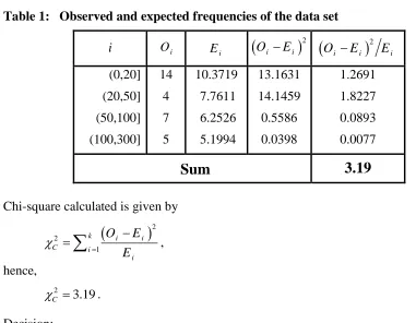
Table 1: Observed and expected frequencies of the data set
i Oi Ei
2
i i
O E
Oi Ei
2 Ei(0,20]
(20,50]
(50,100]
(100,300] 14
4
7
5
10.3719
7.7611
6.2526
5.1994
13.1631
14.1459
0.5586
0.0398
1.2691
1.8227
0.0893
0.0077
Sum
3.19
Chi-square calculated is given by
22
1
k i i
C i
i
O E
E
,hence,
2
3.19
C
.
Decision:
The calculated C2 is 9..3, and the associated p-value is 0.074. Since the p-value is quite high of the significance level 0.05, we cannot reject the null hypothesis that the data are coming from the Weibull distribution.
To show the inference for the unknown parameters of the Weibull distribution under generalized Type-II PHCS, we have n 30, m 10 and the progressively Type-II censored sample obtained from data on the failure times can be reported in Table 2:
Table 2: The progressively Type-II censored sample obtained from the data set on the failure times in the life test
i 1 2 3 4 5
6 7 8 9 10
i
x 1 7 11 14 20 47 71 87
95 246 Ri 2 2
2 2 2 2 2
2 2 2
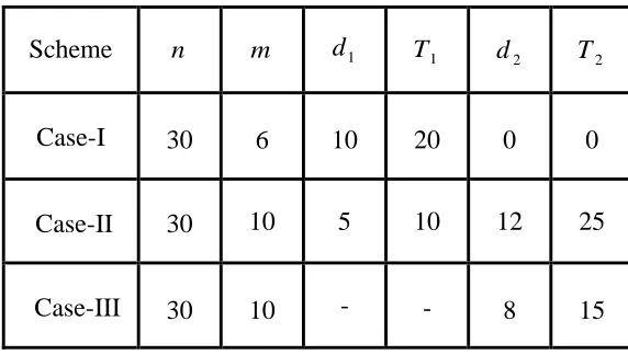
Table 3: Design the progressively Type-II censored sample obtained from the data set on the failure times under generalized Type-II PHCS
Scheme n m d1 T1 d2 T2
Case-I 30 6 10 20
0 0
Case-II 30 10 5 10 12 25
Case-III 30 10 - - 8 15
In Table 3, (-) represent to a number of observed failures which not more than d2.
Using Table 3 to compute the present new results of Weibull distribution based on generalized Type-II PHCS as follows:
(a) Using R statistical programming language with ‘maxLik’ package, the maximum likelihood estimates, the confidence intervals for Weibull parameters under generalized Type-II PHCS and the corresponding elements of inverse Fisher information matrix are calculated, (see Table 4).
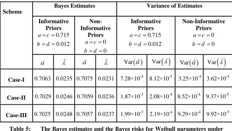
(b) Using MATHCAD package version 2007 and the posterior distribution in the case of Weibull distribution (15), the Bayes estimates and Bayes risks for Weibull parameters are calculated, (see Table 5).
6. Conclusions
Scheme
Maximum Likelihood Estimates
Variance & Covariance of Estimates
Confidence Intervals
ˆ
ˆ Var
ˆ Var
ˆ Cov
ˆ,ˆ
L U L U
Case-I
1.0947 0.0074 0.0477 5.22e-05 -0.0015 0.6664 1.5229 0 0.0216Case-II
0.8064 0.0135 0.0403 1.68e-04 -0.0025 0.4129 1.1999 0 0.0389Case-III
1.0212 0.0085 0.0795 9.29e-05 -0.0026 0.4686 1.5739 00.0274
Table 4: The maximum likelihood estimates and approximate 95% two sided confidence intervals for Weibull parameters under generalized Type-II PHCS
Scheme
Bayes Estimates Variance of Estimates
Informative Priors
0.715
0.012
a c
b d
Non-Informative
Priors
0
0
a c
b d
Informative Priors
0.715
0.012
a c
b d
Non-Informative Priors
0
0
a c
b d
Var
Var
Var
Var
Case-I 0.7063 0.0235 0.7075 0.0231 7.28×10⁻⁴ 8.12×10⁻⁵ 3.25×10⁻⁴ 3.62×10⁻⁵
Case-II 0.7029 0.0246 0.7059 0.0236 1.87×10⁻³ 2.08×10⁻⁴ 8.52×10⁻⁴ 9.37×10⁻⁵
Case-III 7.0025 0.0248 0.7057 0.0237 1.99×10⁻³ 2.19×10⁻⁴ 9.29×10⁻⁴ 9.92×10⁻⁵ Table5: The Bayes estimates and the Bayes risks for Weibull parameters under
generalized Type-II PHCS
References
1. Childs, A., Chandrasekar, B. & Balakrishnan, N. (2008). Exact likelihood inference for an exponential parameter under progressive hybrid censoring. In
2. Gupta, R.D. & Kundu, D. (2001). Exponentiated exponential family: an alternative to gamma and Weibull distributions. Biometrical journal, 43, 117-130.
3. Henningsen, A. and Toomet, O. (2011). ‘maxLik’: A package for maximum likelihood estimation in R. Computational Statistics, 26, 443-458.
4. Johnson, N.L., Kotz, S. and Balakrishnan, N. (1994). Continuous Univariate Distributions, Second Edition. John Wiley, New York.
5. Kundu, D. and Joarder, A. (2006). Analysis of Type-II progressively hybrid censored data. Computational Statistics and Data Analysis, 50, 2509-2528.
6. Lee, K., Sun, H. and Cho, Y. (2015). Exact likelihood inference of the exponential parameter under generalized Type-II progressive hybrid censoring.
Journal of the Korean Statistical Society, 45, 123-136.