www.atmos-meas-tech.net/7/3813/2014/ doi:10.5194/amt-7-3813-2014
© Author(s) 2014. CC Attribution 3.0 License.
Quantifying the value of redundant measurements at GCOS
Reference Upper-Air Network sites
F. Madonna1, M. Rosoldi1, J. Güldner2, A. Haefele3, R. Kivi4, M. P. Cadeddu5, D. Sisterson5, and G. Pappalardo1 1Consiglio Nazionale delle Ricerche, Istituto di Metodologie per l’Analisi Ambientale (CNR-IMAA), C. da S. Loja, Tito Scalo, Potenza, 85050, Italy
2Deutscher Wetterdienst, Meteorologisches Observatorium Lindenberg Richard Assmann Observatorium, Am Observatorium 12, 15848 Tauche/Lindenberg, Germany
3Federal Office of Meteorology and Climatology MeteoSwiss, Chemin de l’Aérologie, 1530 Payerne, Switzerland 4Finnish Meteorological Institute, Arctic Research, Tähteläntie 62, 99600 Sodankylä, Finland
5Argonne National Laboratory, 9700 South Cass Avenue, Argonne, IL 60439-4801, USA Correspondence to: F. Madonna ([email protected])
Received: 28 April 2014 – Published in Atmos. Meas. Tech. Discuss.: 23 June 2014
Revised: 11 September 2014 – Accepted: 24 September 2014 – Published: 19 November 2014
Abstract. The potential for measurement redundancy to re-duce uncertainty in atmospheric variables has not been in-vestigated comprehensively for climate observations. We evaluated the usefulness of entropy and mutual correla-tion concepts, as defined in informacorrela-tion theory, for quan-tifying random uncertainty and redundancy in time series of the integrated water vapour (IWV) and water vapour mixing ratio profiles provided by five highly instrumented GRUAN (GCOS, Global Climate Observing System, Ref-erence Upper-Air Network) stations in 2010–2012. Results show that the random uncertainties on the IWV measured with radiosondes, global positioning system, microwave and infrared radiometers, and Raman lidar measurements dif-fered by less than 8 %. Comparisons of time series of IWV content from ground-based remote sensing instruments with in situ soundings showed that microwave radiometers have the highest redundancy with the IWV time series measured by radiosondes and therefore the highest potential to reduce the random uncertainty of the radiosondes time series. More-over, the random uncertainty of a time series from one instru-ment can be reduced by ∼60 % by constraining the mea-surements with those from another instrument. The best re-duction of random uncertainty is achieved by conditioning Raman lidar measurements with microwave radiometer mea-surements. Specific instruments are recommended for atmo-spheric water vapour measurements at GRUAN sites. This
approach can be applied to the study of redundant measure-ments for other climate variables.
1 Introduction
The use of redundant measurements is considered the best approach to reduce the uncertainty of an atmospheric vari-able. For this reason, several atmospheric observatories have extended their observing capabilities and have acquired mul-tiple instruments that measure the same atmospheric vari-ables with different measurement techniques and retrieval al-gorithms.
Redundancy can be defined as the duplication or the mul-tiplication of the estimation of an atmospheric variable with the aim of increasing reliability in the study of the same vari-able over the time. Without doubt, redundant measurements provide added value towards the full exploitation of the syn-ergy among different measurements techniques: the main ad-vantages are related to
– filling gaps and improving measurement continuity over time and vertical range;
– addressing instrument noise and identifying possible bi-ases or retrieval problems by comparing different tech-niques and instruments.
Comprehensive studies to quantify the effective value of re-dundant measurements and their ability to reduce uncertainty of essential climate variables (ECVs), as retrieved by multi-ple ground-based techniques and in situ active and passive remote sensing, are missing. To this end, GRUAN (GCOS, Global Climate Observing System, Reference Upper-Air Network) aims at providing long-term, highly accurate measurements of atmospheric profiles, complemented by surface-based state-of-the-art instrumentation, for full char-acterization of ECVs and their changes in the complete at-mospheric column (Seidel et al., 2009; Thorne et al., 2013). GRUAN, which is now being implemented, is aimed at sup-porting a network of 30–40 high-quality, long-term upper-air observing stations, building on existing observational net-works.
Cross-checking of redundant measurements for consis-tency is an essential part of the GRUAN quality assurance procedures. A fully equipped GRUAN site should make at least three redundant measurements of all GCOS ECVs (Sei-del et al., 2008). As a consequence, the GRUAN commu-nity has fostered GATNDOR (GRUAN Analysis Team for Network Design and Operations Research), a scientific team charged with addressing key scientific questions of major in-terest to GRUAN and identifying reliable metrics for quanti-fying the value of redundant measurements.
The present study used observations of the vertical-profile of water vapour mixing ratio and the integrated water vapour (IWV) content from a few GRUAN sites equipped with ra-diosondes, global positioning system (GPS), lidars, radiome-ters, spectromeradiome-ters, and radars. Studies of redundant mea-surements should be based on the preliminary identification of a reliable metric. Linear correlation (Pearson’s or Spear-man’s) has typically been used to study redundant measure-ments and their reliability. More recently, Fassò et al. (2014) presented a new approach for an advanced statistical mod-elling based on functional data analysis of the relationships among collocation uncertainty and a set of environmental factors (e.g. wind speed and wind direction). The approach, which can decompose the total collocation uncertainty, could be adapted to evaluate the measurement redundancy. In this paper, we present the results of the GATNDOR study of re-dundant measurements at GRUAN sites. The present study identifies mutual correlation (MC), which is related to the concept of entropy, as a suitable metric for quantifying the value of measurement redundancy. In information theory, en-tropy is a measure of the probabilistic uncertainty associated with a random variable. The approach presented here repre-sents a fast, efficient way to quantify the value of redundant measurements and to correlate the value with factors such as number of instruments, as reported in this work, type of measurement techniques, and retrieval algorithms.
The aims of the paper are
– to show the potential of entropy and MC as metrics for quantifying uncertainty (in a probabilistic sense) and the value of redundancy in climate time series;
– to study, according to GRUAN standards, the uncer-tainty and the value of redundancy of in situ and ground-based remote sensing techniques for estimating ECVS; – to provide the GRUAN community and others interested in the observation of atmospheric thermodynamics with recommendations for the establishment of an observa-tion protocol to reduce the uncertainty of a measurement time series through measurement redundancy;
– to aid site scientists, managers, and funders in making informed decisions on new instrument procurements to maximize the scientific return on the capital expendi-ture.
Section 2 outlines information theory concepts used for the study of redundancy and presents the data sets consid-ered in this work. The data sets were provided by five can-didate GRUAN sites: the Atmospheric Radiation Measure-ment (ARM) Program Southern Great Plains in Oklahoma, USA (Miller et al., 2003); CIAO (Consiglio Nazionale delle Ricerche, Istituto di Metodologie per l’Analisi Ambientale (CNR-IMAA) Atmospheric Observatory) in Potenza, Italy (Madonna et al., 2011); Lindenberg in Germany (Adam et al., 2005); Payerne in Switzerland (Calpini et al., 2011); and Sodankylä in Finland (Hirsikko et al., 2014). Section 3 pro-vides results and preliminary remarks on the value of redun-dant measurements in reducing uncertainty and introduces a possible criterion for addressing redundancy in the frame of GRUAN. Section 4 summarizes the conclusions.
2 Methodology
2.1 Comparison methods
Comparisons among time series of in situ and ground-based remote sensing measurements have been performed mostly by using the concept of variance and root-mean-square dif-ference, less frequently in terms of “information” content (e.g. Majda and Gershgorin, 2010). In information theory, as in thermodynamics, entropy is a measure of the number of specific ways a system can be arranged. Entropy is often con-sidered a measure of disorder or uncertainty in the outcome or the prediction of an event. Commonly used in time series analysis is the Shannon–Wiener entropy measure (Cover and Thomas, 1991). Givenx events in the populationX occur-ring with probabilitiesp(x), the Shannon entropy is defined as
H (x)= −X
x∈X
Therefore,His a measure of probabilistic uncertainty or dis-persion of the probabilities of events. The entropy is calcu-lated from a histogram of probabilities; it has a maximum value if all measurements have equal probability of occur-rence and a minimum value of 0 if the probability of one measurement is 1 and the probability of all the others is 0. TheH is not equivalent to variance (σ), though for particu-lar classes of distributions (e.g. Gaussian),His simply some function ofσ, and they can be considered almost equivalent. Entropy generalizes the concept of measurement uncertainty for calculations of MC. NormalizedH is used here to quan-tify the uncertainty of a time series, andH is normalized by dividingHby the logarithm of the number of states (i.e. the number of possible entries in the related histogram).
In information theory, MC is a measure of the statisti-cal dependence of two random variables or, equivalently, the amount of information that one variable contains about the other (Cover and Thomas, 1991). The MC value can be con-sidered a qualitative indication of how well one measurement explains the other. This means that MC quantifies the reduc-tion of uncertainty in a variableY after one observes another variableX. The advantage in using MC with respect to Pear-son’s or Spearman’s correlation coefficient (ρ) is that MC is a more general measure thanρ, because it does not assume linear or even monotonic correlation. Entropy and mutual in-formation are both rather insensitive to outliers, but even a single outlier can arbitrarily impact both the variance and correlation between two distributions, obscuring the similar-ity of two closely related variables.
The MC of two discrete random variablesXandY can be defined as (Cover and Thomas, 1991)
MC(X, Y )=X
y∈Y X
x∈X
p (x, y)log p (x, y) p (x) p (y)
, (2)
wherep(x, y)is the joint probability distribution function of XandY, andp(x)andp(y)are the marginal probability dis-tribution functions ofXandY, respectively. For continuous random variables, the summation is implemented with a defi-nite double integral. The redundancy concept is a generaliza-tion of mutual informageneraliza-tion toN variables (X1,X2, . . ., XN). Given as marginal entropies H (X)andH (Y ), MC can be also defined as
MC(X, Y )=H (X)+H (Y )−H (X, Y ). (3) The joint entropy H (X, Y )is the total amount of informa-tion for two time series and is calculated by using the joint histogram of the two series. If the two measurements are totally unrelated, then the joint entropy will be the sum of the entropies of the individual measurements. In general, H (X, Y )≤H (X)+H (Y ). The entropy gained from a mem-ber of a mixture of distributions is the difference between the entropy of the average distribution and the average of the entropies of the individual distributions.H (X, Y )can be cal-culated by using the joint histogram ofXandY.
The MC can be also linearized; differences between non-linear and non-linear redundancy provide a qualitative test for the non-linearity of the investigated problem. The linear MC is defined as (Cover and Thomas, 1991)
LMC=1
2 m X
i=1 Cii−1
2 m X
i=1
λCi , (4)
where theCii values are the diagonal elements of the co-variance matrix C of themtime series investigated, and the λ values are the eigenvalues of C. A comparison between linear and non-linear MC is in Sect. 3.4.
Many applications require a metric – a distance measure not only between points but also between data clusters (or time series of data). Different distances are defined in the literature (Arkhangel’skii and Pontryagin, 1990). Here,Dis defined as
D(X, Y )=1−MC(X, Y )/max(H (X), H (Y )), (5) whereDis a metric that satisfies the triangle inequality (i.e. givenX,Y,Z, the sum ofD of any two of the considered variables must be greater than or equal to the value ofDfor the remaining variable). Calculation of MC is an effective way to compare clustering and study relationships between time series (Correa and Lindstrom, 2012).
Finally, the conditional entropy is defined asH (X|Y )=
H (Y )−MC(X, Y ). This definition can be generalized for two or more conditioning variables through the chain rule for joint entropy (Cover and Thomas, 1991).
2.2 Data sets and instruments
on the integrated water vapour content achievable with mi-crowave radiometers and profilers is strongly dependent on the retrieval types, but it is typically within about±0.07 cm; the GPS uncertainty on the integrated water vapour content is typically within about±0.15 cm (first results from GRUAN comparisons with CFH). GRUAN is establishing a database of ECV measurements from the different techniques and in-struments, including full characterization of the uncertainty budget (random and bias contributions). The added value of GRUAN products is related to the implementation of data processing including several corrections for spurious effects on the radiosonde measurements and therefore on the fidelity of the long-term records of radiosondes used for climate ap-plications (Immler et al., 2010; Immler and Sommer, 2010). At present, only quality-assured measurements obtained by RS92-SGP sondes are flowing into the GRUAN data archive. Unfortunately, the approach presented in this paper cannot be used to show the advantages of using GRUAN sonde prod-ucts, mainly because the bias component of the total uncer-tainty budget cannot be quantified through the entropy anal-ysis presented here.
Water vapour measurements from sensors not considered in this study are also available for the considered sites (as noted in Table 1); they are a subject for future study. The current water vapour measurements were selected according to data availability for each site. A similar investigation could be performed for other ECVs. For coherency, we used sonde data processed at each site rather than GRUAN products, which are still not available at all sites and for all radiosonde types. Moreover, retrieval algorithms for passive instruments usually take advantage of historical radiosonde data sets as a statistical constraint.
Simultaneous data from all available instruments were se-lected according to the conditions of clear sky (per lidar mea-surements or radiosonde humidity), nighttime, and, if lidar data are available, a relative error of lidar water vapour mix-ing ratio at 7 km a.g.l. <25 %. This error is considered a good compromise having an adequate lidar signal-to-noise ratio and also covering the part of the troposphere where most of the water vapour can be observed. Raman lidar mea-surements are integrated over 10 min around the sonde syn-optic launch time to keep a good signal-to-noise ratio in the investigated region, and MWR and microwave profiler mea-surements are provided every 10 min. GPS data are provided only every 15 min, because of constraints on data processing at the considered sites, and the closest measurements to the sonde launch time (within 10 min) are compared. The use of MWR to calibrate the ARM Raman lidar measurements af-fects the independence of the IWV comparison for lidar at the SGP; in contrast, at Payerne and Potenza the Raman lidar is calibrated by using radiosonde humidity profiles in the lower troposphere (Madonna et al., 2011; Brocard et al., 2013).
Data from different sites are currently processed with dif-ferent algorithms; this could affect the comparison. However, the study of entropy is also a good check for the effect of
re-trieval inconsistencies. A linear regression on the entire time series (3 years) of IWV data and vertical profiles of water vapour mixing ratio at the altitude levels removed natural or artificial trends (e.g. calibration drifts). This was done to sup-press the bias component of the time series uncertainty and to ensure that the reported entropies are related only to the random uncertainty.
2.3 Optimal binning choice and minimally sufficient data
The two crucial issues that need to be considered for entropy calculation using the histogram of a variable are the minimal quantity of data required to reduce inaccuracies in the calcu-lation and the choice of the optimal binning to represent the actual probability density functions (PDFs) of the variable.
To make our histogram representative of the real un-derlying PDF of the variable and to calculate the re-lated entropy, a minimal number of data points is needed. The data sets considered here include >140 cases per station (Lindenberg = 296, Payerne = 174, Southern Great Plains = 144). For Potenza and Sodankyla, more restricted data sets (40 and 22 cases, respectively) were used, because of the unique sampling strategy at Potenza (one radiosonde launch per week, only in clear sky) and the limited number of cryogenic frost point hygrometer (CFH) launches made available by Sodankyla for this study. Knuth (2013) reported that at least 100 cases should be considered to avoid under-estimation of entropy, though the number might depend on the underlying distribution. Nevertheless, values of the en-tropy calculated for Potenza and Sodankyla are quite similar to those reported for other sites. This is encouraging, though a margin of inaccuracy affecting the values can be quanti-fied only if larger data sets become available for the specific instruments at both stations.
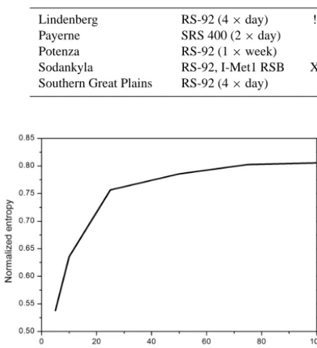
To determine the optimal binning, several statistical meth-ods have been proposed (Knuth, 2013). In Fig. 1, entropy is shown as a function of the number of bins used to build the histogram for the Payerne radiosonde data sets. The value of entropy increases up to 0.81 for a histogram with 100 bins. Between 25 and 100 bins, entropy tends to assume asymp-totic behaviour. In this work, in view of the behaviour shown in Fig. 1 and the number of data points available, 50 bins per histogram are used.
3 Results and discussion
Table 1. Instruments available (and model when applicable) at the GRUAN sites generating data sets considered in this study of uncertainty
and redundancy. Symbol ! indicates that the instrument is available at the site, but the data were not used in the study. Abbreviations: CFH, cryogenic frost-point hygrometer; MWR, microwave radiometer; MWP, microwave profiler; GPS, global positioning system; FTIR, Fourier transform infrared radiometer; AERI, atmospheric emitted radiance interferometer.
GRUAN site/instrument Sonde CFH Lidar MWR MWP GPS FTIR
Lindenberg RS-92 (4×day) ! X Radiometrics Radiometrics GFZ Payerne SRS 400 (2×day) X HATPRO GFZ Potenza RS-92 (1×week) X Radiometrics !
Sodankyla RS-92, I-Met1 RSB X ! ! Bruker Southern Great Plains RS-92 (4×day) X Radiometrics Suominet AERI
Figure 1. Entropy as a function of the number of bins used to build
the histogram for the Payerne radiosonde.
all contributions affecting the uncertainty of a measurements time series – sampling uncertainty, uncertainty due to the time and vertical average, atmospheric variability, and all other relevant environmental factors (Kitchen, 1989; Fassò et al., 2014), such as solar radiation affecting daytime in situ soundings.
Figure 2 (left) is an example of a series of samples of the IWV for the Lindenberg instruments (Table 1), while Fig. 2 (right) shows the corresponding histograms of the time series. After linear detrending of the time series described above, the histograms were used to calculate entropy and MC. The shape of the histograms in Fig. 2 clarifies both how outliers can occur by chance in any distribution, often indi-cating either measurement errors or a heavy-tailed distribu-tion in the populadistribu-tion, and also the absence of any guarantee that the distribution will be a normal one. The discrepancies between the time series reported in Fig. 2 (left) translate into a sort of bi-modal distribution characterized by a high kur-tosis (Fig. 2, right). Thus, caution is needed in assuming a normal distribution; statistics, like entropy, that are robust to outliers and independent on the underlying distribution are more reliable for characterizing the uncertainty of a time se-ries.
To show the reader the advantages of using entropy and MC instead of using standard deviation (σ) andρ, we show in Fig. 3 a Taylor diagram (left panel) obtained from the GPS IWV time series collected at Lindenberg, and the same time series but adding to the IWV probability density function 5, 10, 20, 30, and 40 outliers respectively. The correlation has been calculated with respect to an underlying Gaussian dis-tribution fitted to the data. The value of theσ in the diagram obtained from the original time series is reported as the “ob-served” curve. Taylor diagrams provide a concise statistical summary of the similarity between two patterns, quantified in terms of their correlation, their centred root-mean-square difference and the amplitude of their variations (represented by theirσs). These diagrams are especially useful in evalu-ating multiple aspects of complex models or in gauging the relative skill of many different models or measurement tech-niques.
Following previous studies, the Taylor diagram described above is compared in Fig. 3 with a modified Taylor dia-gram (Correa and Lindstrom, 2012) obtained by replacing the standard deviation with the entropy andρwith MC (right panel). Mutual correlation was also calculated with respect to an underlying Gaussian distribution. The comparison clearly shows that entropy and, accordingly, MC are much more in-sensitive thanσ andρto outliers applied to the original dis-tribution of GPS IWV data. This supports the use of entropy and MC as tools to analyse a data set without the need to make assumptions on the underlying distribution function. 3.1 Normalized entropy for integrated water vapour
and vertical profiles
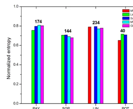
Figure 4 compares the normalized entropiesH /logn, where n is the number of states (histogram entries) retrieved for all instruments measuring IWV at the Lindenberg, Payerne, Potenza, and Southern Great Plains sites. For Lindenberg, Payerne, and Southern Great Plains at least four instruments are available; for Potenza, GPS IWV is available only from June 2011 and thus is not included in this study.
Figure 2. Example of the time series (left) of integrated water vapour obtained with the instruments available at the Lindenberg site (reported
in Table 1) and histograms (right) of the time series shown in the left panel. After detrending of the time series, the histograms were used to calculate entropy and mutual correlation.
Figure 3. The left panel shows a Taylor diagram obtained for the
GPS IWV time series collected at Lindenberg, and the same time series but adding to the IWV probability density function 5, 10, 20, 30, and 40 outliers respectively. The correlation has been calculated with respect to an underlying Gaussian distribution fitted to 637 the data; in the right panel, a modified Taylor diagram is obtained by replacing the standard deviation with the entropy andρwith MC.
With the exception of Payerne, lidar entropy is the closest to radiosonde entropy, whether calibrated by using the sonde it-self or the MWR. Moreover, at Payerne the lidar offers the lowest entropy of the instrument ensemble. At the SGP, GPS has the lowest entropy, though the values for all considered instruments are quite close. Similarly, at Lindenberg, where the MWR has the lowest entropy, all values are similar. At Potenza, the lowest entropy value is for the microwave pro-filer. As a whole, differences in the entropy of the time series between the different instruments are within 8 %. Obviously, the different atmospheric variability of each site can also re-sult in large deviations between entropy values. This devi-ation could be smoothed if a longer temporal data set was investigated. Moreover, differences in the observation tech-niques and their experimental implementation (e.g. different measurement angles and fields of view) might also contribute to differences in the calculated entropies and to non-linear calibration drifts.
Figure 4. Comparison of the normalized entropy retrieved for the
instruments measuring integrated water vapour at the Lindenberg (LIN), Payerne (PAY), Potenza (POT), and Southern Great Plains (SGP) sites. The data set considered includes all available mea-surements in 2010–2012. The numbers above the bars represent the number of cases selected, according to the quality assurance criteria for each station.
3.2 Mutual correlation and distance for integrated water vapour and vertical profiles
Figure 5. Comparison of the statistical distances between pairs of
times series data retrieved for the instruments measuring integrated water vapour with respect to the time series obtained from the ra-diosondes at the Lindenberg (LIN), Payerne (PAY), Potenza (POT), and Southern Great Plains (SGP) sites. The data set considered in-cludes all available measurements in 2010–2012.
from the radiosonde series are >0.18 for lidar,>0.32 for GPS,>0.14 for MWR, and>0.28 for microwave profiler. At Payerne and Potenza, all the techniques show good re-dundancy, though GPS IWV at Potenza is not included in the statistics, because the number of measurements is small for the considered period. However, criteria are needed to de-termine the acceptable levels of uncertainty and redundancy for a climate observation network. Section 3.5 deals with this aspect in more detail.
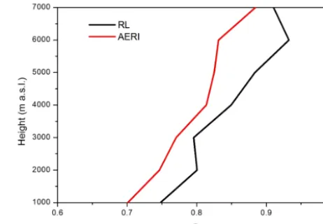
Normalized entropy and MC are compared for the avail-able measurements of the water vapour or relative humid-ity (RH) vertical profiles. In Fig. 6, the distance of the water vapour vertical profiles obtained with the Raman li-dar (RL) and atmospheric emitted radiance interferometer (AERI) with respect to radiosonde (RS92) profiles are com-pared. Lidar profiles were retrieved by integrating signals over 10 min around the sonde launch time. The AERI pro-files were averaged in the same time window. To improve the comparison among in situ, active and passive remote sensing measurements, the profiles from the three instruments were averaged over a vertical range of 1 km. This should strongly reduce the differences related to instrument signal-to-noise ratio and to the effective vertical resolution, which differs for the different techniques. Moreover, for the AERI, the sta-tistical retrieval provided by the ARM Archive (Turner and Loehnert, 2014) was considered; this retrieval is based on the radiosonde profile as a first guess, which affects the calcula-tion of distance. Nevertheless, the comparison is provided to test the approach for passive profile retrievals. Figure 6 shows that, though the difference is small, AERI has lower values of distance along the entire profile, probably because of the use
Figure 6. Comparison of the statistical distances of the Raman lidar
(RL) and the atmospheric emitted radiance interferometer (AERI) time series from the RS92 radiosonde time series of water vapour vertical profile at the Southern Great Plains (SGP) site. The data set considered includes all measurements available at the SGP in 2010–2012, in 144 profiles.
of collocated radiosonde data as first guesses in the retrieval algorithm.
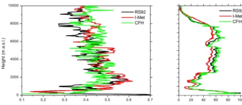
Figure 7. Comparison of the normalized entropy values (left) for
the RS92 and Intermet radiosondes (I-Met) and the cryogenic frost-point hygrometer (CPH) measuring the in situ water vapour vertical profile at the Sodankyla site in 2010 (left panel); comparison of the relative humidity profiles in one case on 15 March 2010 (right panel).
the total uncertainty budget. This contribution can, in princi-ple, be modelled and removed, but because of its systematic nature it cannot be evaluated with the entropy analysis dis-cussed here. The presented analysis allows us only to state that the RH time series measured by the RS92, I-Met, and CFH show similar random uncertainty at all altitude levels below 10 km.
3.3 Conditional entropy
The conditional entropy quantifies the amount of informa-tion needed to describe the outcome of a random variableY, given the value of another random variableX. The condition-ing usually reduces entropy. That is, given two time seriesX and Y, the conditional entropy H (X|Y )≤H (X). Equality occurs only ifXandY are fully independent. Figure 8 shows the values of conditional entropy retrieved for most of the possible combinations of instruments measuring IWV at the SGP (upper panel) and POT (bottom panel) sites, for the data sets described above. In both plots, the values of the nor-malized entropies calculated for each single instrument are also shown as a comparison term to quantify the residual un-certainty affecting each instrument when one or more other instruments are assumed as good constraints. Figure 8 shows that the residual entropy obtained by conditioning one in-strument with a second inin-strument is 30–40 % lower than the entropy obtained for a single instrument. If two instruments are used for the conditioning, the residual entropy ranges be-tween 5 and 20 %. This finding indicates that with reliable constraints, the entropy can be reduced by about 60–65 % with respect to the use of a single instrument. The minimum residual uncertainties are obtained when the GPS is condi-tioned with the RL and the MWR at the SGP site, and when the RL is conditioned with the microwave profiler at the POT site.
These results also show that the residual uncertainties ob-tained with two conditioning constraints (two instruments) can be better than or similar to the value with only one
instru-Figure 8. Comparison of the normalized conditional entropy values
retrieved for most of the possible combinations of instruments mea-suring integrated water vapour at the Potenza site (upper panel) and the Southern Great Plains site (bottom panel).
ment as a constraint. This is relevant when synergetic prod-ucts must be defined and retrieved by using algorithms that can integrate information from ground-based or satellite sen-sors. This is the case for all optimal estimation algorithms based on the Bayes’ theorem, which is frequently adopted to improve atmospheric profiling. To quantify the effective advantages of integration, the presented analysis can be per-formed in advance of the elaboration of algorithms integrat-ing measurements from different sensors. Moreover, condi-tional entropy can be applied similarly for directly measured quantities, like radiances, as well as for data products such as water vapour ground-based remote sensing. This is the case for algorithms making use of satellite measurements from polar and geostationary satellites to improve the resolution or reduce the uncertainty affecting the estimation of ECVs, but it is also true for algorithms merging satellite and ground-based passive sensor data to improve atmospheric profiling. 3.4 Linear mutual correlation
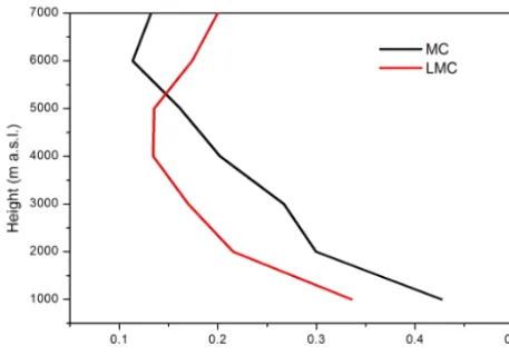
Figure 9. Comparison of the normalized mutual correlation for the
linear (LMC) and non-linear cases (MC), calculated for the lidar and radiosonde data sets from the Potenza site.
LMC for quantifying the value of redundant measurements. The result is in agreement with outcomes from previous stud-ies that analysed data sets including different types of data and compared Taylor’s diagrams built by using standard de-viation versus correlation and entropy versus MC (e.g. Cor-rea and Lindstrom, 2012).
3.5 Redundancy criteria
The analysis above shows how to approach the problem of quantifying measurement redundancy by using the concepts of information theory. However, the usefulness of this ap-proach can be clarified only if some criteria are identified to classify when two data sets are redundant. This obviously depends on the investigated variable and on the uncertainty limits assumed to be minimum requirements for studying a certain atmospheric process or climate trend.
Here, we present an example showing the relationship be-tween distance values and the random uncertainty affecting IWV measurements. The aim is to clarify the use of MC and the related distance for quantifying redundant IWV measure-ments at GRUAN sites. The plot of Fig. 10 shows the dis-tance between the radiosonde IWV time series at Lindenberg and the corresponding time series obtained by adding vari-able random noise to the radiosonde time series. The random noise is added to reproduce the effect of an additional ran-dom uncertainty, with relative values of 0–100 % affecting an IWV time series with respect to the reference series. For example, a distance value lower than about 0.2 corresponds to a random uncertainty 20 % larger than that of the original time series assumed as the reference. This example indicates a very simple way to approach data sets from different instru-ments or techniques, fixing a threshold consistent with the desired redundancy requirements. According to the GCOS requirements for the state-of-art capability, also reported in the GRUAN manual (http://www.wmo.int/pages/prog/gcos/
Figure 10. Statistical distance between the integrated water vapour
time series retrieved from the radiosonde at the Lindenberg site and the corresponding time series obtained by adding random noise to the radiosonde time series to simulate the effect of increasing rela-tive random uncertainty.
publications/gcos-171.pdf), atmospheric water vapour must be measured with a random error<5 % in the entire tropo-sphere and stratotropo-sphere. This corresponds to a maximum ran-dom error<5 % affecting an IWV time series. If the random uncertainty is quantified by using entropy and the radiosonde IWV time series (the reference) is affected by random errors <5 %, an IWV time series affected by a random error<5 % is consistent with the true series if the corresponding distance value is lower than about 0.2 (total random error <10 %). The plot in Fig. 5 shows that the distance values for different instrument and different sites do not always meet this stan-dard. The values>0.2 should be classified as not redundant in terms of the threshold of 5 % random error affecting the two compared time series.
4 Conclusions
The ultimate aim of this study is to recommend the best combination of instruments for monitoring atmospheric wa-ter vapour. Though entropy and MC are robust concepts pro-vided in information theory, representing appropriate metrics to quantify the uncertainty and redundancy of atmospheric measurements, they have never been applied extensively to climate data. In this paper, we show how entropy and MC can be used to evaluate the random probabilistic uncertainty in the ECV by analysing measurement redundancy.
The following conclusions can be drawn from the results of this study of data sets of water vapour from five GRUAN observation stations in 2010–2012:
(Raman lidar, GPS, MWR, microwave profiler, sondes) differs by<8 %.
2. In terms of the best performances for each instrument at the different sites, the comparison of IWV time se-ries showed that MWR have the highest redundancy and therefore the highest potential to reduce the random un-certainty of IWV time series as measured by radioson-des.
3. The distance between the time series of water vapour profiles at each altitude level has been also performed to show how to evaluate the redundancy of collocated in situ, active and passive profiling instruments, though for passive instruments this also depends on the retrieval algorithms and on which first-guess prior covariance is used.
4. Both RS92 and I-Met radiosondes can measure in situ atmospheric water vapour with the same random uncer-tainty as the CFH, though the sondes are affected by a bias error that cannot be evaluated with the present ap-proach.
5. A conditional entropy analysis showed that condition-ing of the time series with more than one instrument, assumed as constraints, can decrease the residual en-tropy by at least 60 % versus the use of one conditioning instrument. Moreover, the use of two conditioning in-struments versus one results in similar or slightly better residual uncertainty.
6. An analysis of the relationship between distance and the random uncertainty showed that a maximum random er-ror <5 % affecting the IWV estimated by two differ-ent techniques corresponds to a distance value less than about 0.2. That is, an IWV time series whose distance from a reference time series (i.e. IWV measured by ra-diosondes) is>0.2 exceeds the redundancy limits iden-tified according to the GCOS criteria.
Final recommendations can be provided only if criteria to support a certain network are clearly defined according to the uncertainty thresholds assumed in the study of an ECV; how-ever, the presented approach is versatile enough to be used with different data sets, stations, and instruments to provide the required feedback in terms of uncertainty and use of re-dundant measurements to reduce uncertainty in ECV values. As a whole the concepts of entropy and mutual correlation demonstrate their potential if used as metrics for quantifying random uncertainty and redundancy in time series of atmo-spheric observations. The examples discussed in this work support the use of the mutual correlation as a more general concept than other linear metrics for the study of redundant measurements. Moreover, the analysis based on the entropy, MC and conditional entropy can be used for a preliminary
feasibility study of the effective advantages obtained in us-ing retrieval algorithms integratus-ing measurements provided by different observation platforms, ground-based or satellite, both for direct measurements (e.g. radiances) and retrieved products (e.g. temperature, water vapour content, aerosol op-tical depth). For example, this is the case of those algorithms integrating measurements from different sensors using the Bayes’ theorem (that is based on the concept of conditional probability) as well as for those algorithms integrating ra-diances measured by different sensor in different spectral ranges (e.g. Romano et al., 2007).
Acknowledgements. Data sources were as follows: ARM SGP data through the US Department of Energy (www.arm.gov); CIAO Potenza data through CNR-IMAA (http://www.ciao.imaa.cnr.it); Lindenberg data through the Lindenberg Meteorological Ob-servatory, Richard Assmann Observatory, Deutscher Wet-terdienst (http://www.dwd.de); PAY data through the Fed-eral Office of Meteorology and Climatology MeteoSwiss (http://meteoswiss.admin.ch); SOD data through the Finnish Mete-orological Institute (http://www.fmi.fi). The authors also gratefully acknowledge the useful comments of A. Fassò from University of Bergamo. This work was supported by the US Department of Energy, Office of Science, Office of Biological and Environmental Research, under contract DE-AC02-06CH11357. The authors also acknowledge financial support for the ACTRIS Research Infrastructure Project supported by the European Union Seventh Framework Programme (FP7/2007-2013) under grant agreement no. 262254.
Edited by: K. Kreher
References
Adam, W., Dier, H., and Leiterer, U.: 100 years aerology in Lindenberg and first long-time observations in the free atmo-sphere, Meteorol. Z., 14, 597–607, 2005.
Arkhangel’skii, A. V. and Pontryagin, L. S.: General Topology I: Basic Concepts and Constructions Dimension Theory, Ency-clopaedia of Mathematical Sciences, Springer, 1990,
Brocard, E., Philipona, R., Haefele, A., Romanens, G., Mueller, A., Ruffieux, D., Simeonov, V., and Calpini, B.: Raman Lidar for Meteorological Observations, RALMO – Part 2: Validation of water vapor measurements, Atmos. Meas. Tech., 6, 1347–1358, doi:10.5194/amt-6-1347-2013, 2013.
Calpini, B., Ruffieux, D., Bettems, J.-M., Hug, C., Huguenin, P., Isaak, H.-P., Kaufmann, P., Maier, O., and Steiner, P.: Ground-based remote sensing profiling and numerical weather predic-tion model to manage nuclear power plants meteorological surveillance in Switzerland, Atmos. Meas. Tech., 4, 1617–1625, doi:10.5194/amt-4-1617-2011, 2011.
Correa, C. and Lindstrom, P.: The Mutual Information Diagram for Uncertainty Visualization, International Journal for Uncertainty Quantification, 3, 187–201, 2012.
Dirksen, R. J., Sommer, M., Immler, F. J., Hurst, D. F., Kivi, R., and Vömel, H.: Reference quality upper-air measurements: GRUAN data processing for the Vaisala RS92 radiosonde, Atmos. Meas. Tech. Discuss., 7, 3727–3800, doi:10.5194/amtd-7-3727-2014, 2014.
Fassò, A., Ignaccolo, R., Madonna, F., Demoz, B. B., and Franco-Villoria, M.: Statistical modelling of collocation uncertainty in atmospheric thermodynamic profiles, Atmos. Meas. Tech., 7, 1803–1816, doi:10.5194/amt-7-1803-2014, 2014.
Hirsikko, A., O’Connor, E. J., Komppula, M., Korhonen, K., Pfüller, A., Giannakaki, E., Wood, C. R., Bauer-Pfundstein, M., Poikonen, A., Karppinen, T., Lonka, H., Kurri, M., Heinonen, J., Moisseev, D., Asmi, E., Aaltonen, V., Nordbo, A., Rodriguez, E., Lihavainen, H., Laaksonen, A., Lehtinen, K. E. J., Lau-rila, T., Petäjä, T., Kulmala, M., and Viisanen, Y.: Observing wind, aerosol particles, cloud and precipitation: Finland’s new ground-based remote-sensing network, Atmos. Meas. Tech., 7, 1351–1375, doi:10.5194/amt-7-1351-2014, 2014.
Immler, F. and Sommer, M.: GRUAN-TD-4 Brief Description of the RS92 GRUAN Data Product (RS92.GDP), available at: http: //www.gruan.org, last access: 20 June 2014, 2010.
Immler, F. J., Dykema, J., Gardiner, T., Whiteman, D. N., Thorne, P. W., and Vömel, H.: Reference Quality Upper-Air Measure-ments: guidance for developing GRUAN data products, At-mos. Meas. Tech., 3, 1217–1231, doi:10.5194/amt-3-1217-2010, 2010.
Kitchen, M.: Representativeness errors for radiosonde observations, Q. J. Roy. Meteor. Soc., 115, 673–700, 1989.
Knuth, K. H.: Optimal data-based binning for histograms, arXiv preprint physics/0605197, 2013.
Madonna, F., Amodeo, A., Boselli, A., Cornacchia, C., Cuomo, V., D’Amico, G., Giunta, A., Mona, L., and Pappalardo, G.: CIAO: the CNR-IMAA advanced observatory for atmospheric research, Atmos. Meas. Tech., 4, 1191–1208, doi:10.5194/amt-4-1191-2011, 2011.
Majda, A. and Gershgorin, J.: Quantifying uncertainty in climate change science through empirical information theory, P. Natl. Acad. Sci. USA, 107, 14958–14963, 2010.
Miller, M. A., Johnson, K. L., Troyan, D. T., Clothiaux, E. E., Mlawer, E. J., and Mace, G. G.: ARM value added cloud products: Description and status, in: Proc. of the 13th ARM Science Team Meeting, Broomfield, CO, ARM, avail-able at: http://www.arm.gov/publications/proceedings/confl3/ extended_abs/miller-ma.pdf, last access: 20 June 2014, 2003.
Romano, F., Cimini, D., Rizzi, R., and Cuomo, V.: Multilayered cloud parameters retrievals from combined infrared and mi-crowave satellite observations, J. Geophys. Res., 112, D08210, doi:10.1029/2006JD007745, 2007.
Seidel, D. J., Berger, F. H., Diamond, H. J., Dykema, J., Goodrich, D., Immler, F., Murray, W., Peterson, T., Sister-son, D., Sommer, M., Thorne, P., Vömel, H., and Wang, J.: Reference Upper-Air Observations for Climate: Rationale, Progress, and Plans, Bull. Am. Meteorol. Soc., 90, 361–369, doi:10.1175/2008BAMS2540.1, 2009
Suortti, T. M., Kivi, R., Kats, A., Yushkov, V., Kämpfer, N., Leiterer, U., Miloshevich, L. M., Neuber, R., Paukkunen, A., Ruppert, P., and Vömel, H.: Tropospheric Comparisons of Vaisala Radioson-des and Balloon-Borne Frost Point and Lyman-αHygrometers during the LAUTLOS-WAVVAP Experiment, J. Atmos. Ocean. Tech., 25, 149–166, doi:10.1175/2007JTECHA887.1, 2008. Thorne, P. W., Vömel, H., Bodeker, G., Sommer, M., Apituley,
A., Berger, F., Bojinski, S., Braathen, G., Calpini, B., Demoz, B., Diamond, H. J., Dykema, J., Fassò, A., Fujiwara, M., Gar-diner, T., Hurst, D., Leblanc, T., Madonna, F., Merlone, A., Mikalsen, A., Miller, C. D., Reale, T., Rannat, K., Richter, C., Seidel, D. J., Shiotani, M., Sisterson, D., Tan, D. G. H., Vose, R. S., Voyles, J., Wang, J., Whiteman, D. N., and Williams, S.: GCOS reference upper air network (GRUAN): Steps towards as-suring future climate records, AIP Conf. Proc., 1552, 1042–1047, doi:10.1063/1.4821421, 2013.
Turner, D. D. and Loehnert, U.: Information content and uncertain-ties in thermodynamic profiles and liquid cloud properuncertain-ties re-trieved from the ground-based Atmospheric Emitted Radiance Interferometer (AERI), J. Appl. Meteorol. Clim., 53, 752–771, doi:10.1175/JAMC-D-13-0126.1, 2014.
Wang, J., Zhang, L., Dai, A., Immler, F., Sommer, M., and Vömel, H.: Radiation Dry Bias Correction of Vaisala RS92 Humidity Data and Its Impacts on Historical Radiosonde Data, J. Atmos. Ocean. Tech., 30, 197–214, doi:10.1175/JTECH-D-12-00113.1, 2013.