www.the-cryosphere.net/10/811/2016/ doi:10.5194/tc-10-811-2016
© Author(s) 2016. CC Attribution 3.0 License.
Constraining variable density of ice shelves using wide-angle
radar measurements
Reinhard Drews1, Joel Brown2, Kenichi Matsuoka3, Emmanuel Witrant4, Morgane Philippe1, Bryn Hubbard5, and Frank Pattyn1
1Laboratoire de Glaciologie, Université Libre de Bruxelles, Brussels, Belgium 2Aesir Consulting LLC, Missoula, MT, USA
3Norwegian Polar Institute, Tromsø, Norway
4Université Grenoble Alpes/CNRS, Grenoble Image Parole Signal Automatique, 38041 Grenoble, France 5Aberystwyth University, Aberystwyth, Wales, UK
Correspondence to: Reinhard Drews ([email protected])
Received: 23 September 2015 – Published in The Cryosphere Discuss.: 21 October 2015 Revised: 19 March 2016 – Accepted: 31 March 2016 – Published: 15 April 2016
Abstract. The thickness of ice shelves, a basic parameter for mass balance estimates, is typically inferred using hy-drostatic equilibrium, for which knowledge of the depth-averaged density is essential. The densification from snow to ice depends on a number of local factors (e.g., temper-ature and surface mass balance) causing spatial and tempo-ral variations in density–depth profiles. However, direct mea-surements of firn density are sparse, requiring substantial lo-gistical effort. Here, we infer density from radio-wave prop-agation speed using ground-based wide-angle radar data sets (10 MHz) collected at five sites on Roi Baudouin Ice Shelf (RBIS), Dronning Maud Land, Antarctica. We reconstruct depth to internal reflectors, local ice thickness, and firn-air content using a novel algorithm that includes traveltime in-version and ray tracing with a prescribed shape of the depth– density relationship. For the particular case of an ice-shelf channel, where ice thickness and surface slope change sub-stantially over a few kilometers, the radar data suggest that firn inside the channel is about 5 % denser than outside the channel. Although this density difference is at the detec-tion limit of the radar, it is consistent with a similar density anomaly reconstructed from optical televiewing, which re-veals that the firn inside the channel is 4.7 % denser than that outside the channel. Hydrostatic ice thickness calculations used for determining basal melt rates should account for the denser firn in ice-shelf channels. The radar method presented here is robust and can easily be adapted to different radar frequencies and data-acquisition geometries.
1 Introduction
As a snow layer deposited at the ice-sheet surface is progres-sively buried by subsequent snowfall, it transforms to higher-density firn under the overburden pressure. The firn–ice tran-sition, marked by the depth at which air bubbles are isolated, occurs at a density of approximately 830 kg m−3 at depths typically ranging from 30 to 120 m in polar regions (Cuffey and Paterson, 2010, Chapter 2). Densification continues un-til air bubbles transform to clathrate hydrates and pure ice density is reached (ρi≈917 kg m−3). The precise nature of this densification depends on a number of local factors that also vary temporally (Arthern et al., 2010), including surface density and stratification (Hörhold et al., 2011), surface mass balance and temperature (e.g., Herron and Langway, 1980), as well as dynamic recrystallization and the strain regime. Recent studies also highlight the role of microstructure (Gre-gory et al., 2014) and impurities (Hörhold et al., 2012; Fre-itag et al., 2013a, b).
thin-ning (e.g., Wouters et al., 2015); and (iv) to infer ice-shelf thickness for mass balance estimates (Rignot et al., 2013; Depoorter et al., 2013) from hydrostatic equilibrium (Griggs and Bamber, 2011).
Density profiles are most reliably retrieved from ice/firn cores either by measuring discrete samples gravimetrically, or by using continuous dielectric profiling (Wilhelms et al., 1998) or X-ray tomography (Kawamura, 1990; Freitag et al., 2013a). Techniques such as gamma-, neutron-, laser-, or optical-scattering (Hubbard et al., 2013, and references therein) circumnavigate the labor-intensive retrieval of an ice core and only require a borehole, which can rapidly be drilled using hot water.
All of the aforementioned techniques, however, remain point measurements requiring substantial logistics. A com-plementary approach is to exploit the density dependence of radio-wave propagation speed. The principle underlying the technique involves illuminating a reflector with different ray paths such that both the reflector depth and the radio-wave propagation speed may be calculated using methods such as the Dix inversion (Dix, 1955), semblance analysis (e.g., Booth et al., 2010, 2011), interferometry (Arthern et al., 2013), or traveltime inversion based on ray tracing (Zelt and Smith, 1992; Brown et al., 2012).
A typical acquisition geometry is to position receiver and transmitter with variable offsets so that the subsurface reflection point remains the same for horizontal reflectors (common-midpoint surveys, e.g. Murray et al., 2000; Wine-brenner et al., 2003; Hempel et al., 2000; Eisen et al., 2002; Bradford et al., 2009; Blindow et al., 2010). Alternatively, only the receiver can be moved (Fig. 1) resulting in what is sometimes referred to as wide-angle reflection and refraction (WARR; Hubbard and Glasser, 2005, p. 165) geometry. In all cases, density can be inferred from the radar-wave speed using density–permittivity relations (e.g., Looyenga, 1965; Wharton et al., 1980; Kovacs et al., 1995).
Here, we investigate six WARR measurements collected in December 2013 on Roi Baudouin Ice Shelf (RBIS), Dron-ning Maud Land, Antarctica. The WARR sites are part of a larger geophysical survey imaging an ice-shelf pinning-point and a number of ice-shelf channels which are about 2 km wide and can extend longitudinally from the ground-ing line to the ice-shelf front (Le Brocq et al., 2013). Ice inside the channels is thinner, sometimes more than 50 % (Drews, 2015), and the surface is depressed, causing the elongated lineations visible in satellite imagery (Fig. 2). Basal melting inside channels can be significantly larger (Stanton et al., 2013), correspondingly influencing ice-shelf stability (Sergienko, 2013). Adjustment towards hydrostatic equilibrium resulting from basal melting can weaken ice shelves through crevasse formation (Vaughan et al., 2012). Channelized melting, on the other hand, can also prevent excessive area-wide basal melting and hence stabilize ice shelves (Gladish et al., 2012; Millgate et al., 2013).
The basal mass balance inside ice-shelf channels can be mapped from remote sensing assuming mass conservation (e.g., Dutrieux et al., 2013). This approach calculates ice thickness from hydrostatic equilibrium which engenders po-tentially two pitfalls. (i) Bridging stresses can prevent full re-laxation to hydrostatic equilibrium (Drews, 2015), and (ii) it may not account for small-scale variations in material den-sity. Evidence for small-scale changes in density was sug-gested by Langley et al. (2014) and Drews (2015), who found that the surface mass balance can be elevated locally within the concave surface associated with ice-shelf chan-nels, which in turn may impact the local densification pro-cesses. Atmospheric models typically operate with a hori-zontal gridding coarser than 5 km (Lenaerts et al., 2014) and cannot resolve such small-scale variations in surface mass balance and density.
Herein, we calculate densities from WARR sites using traveltime inversion and ray tracing (Sect. 2). The data set is supplemented with densities based on optical televiewing (OPTV) of two boreholes (Fig. 2; Sect. 3). In Sects. 4 and 5, we compare both methods and discuss density anomalies associated with the ice-shelf channels. We present our con-clusions about the derivation of density from radar in general, and the density anomalies in ice-shelf channels in particular in Sect. 6, and discuss consequences of our findings for esti-mating basal melt rates in ice-shelf channels.
2 Development of a new algorithm to infer density from wide-angle radar
We describe the propagation of the radar wave for each off-set as a ray traveling from the transmitter via the reflection boundary to the receiver (Fig. 1). Using a coordinate sys-tem, wherex is parallel to the surface and zpoints verti-cally downwards, the ray paths are determined by the spa-tially variable radio-wave propagation speedv(x, z)which is primarily determined by density; unlessv(x, z)is constant, ray paths are not straight but bend following Fermat’s prin-ciple of minimizing the traveltime between transmitter and receiver. The geometry depicted in Fig. 1 is common in seis-mic investigations, and multiple techniques exist for deriving the velocities from recorded traveltimes (Yilmaz, 1987).
reflec-Figure 1. (a) Plain view of the wide-angle acquisition geometry: transmitting (Tx) and receiving (Rx) antennas were aligned in parallel.
While the transmitter remained at a fixed location, the receiver was incrementally moved farther away. A sketch of the corresponding ray paths is shown in (b) with a synthetic velocity–depth function color coded. The labels of example rays and their incidence angles are presented in Eqs. (1)–(10).
tors from being handed downwards, we refine the method by parameterizing a monotonic depth–density function, and by inverting simultaneously for a set of parameters specifying the density and all reflector depths, described below. 2.1 Experimental setup
The radar consists of resistively loaded dipole antennas (10 MHz) linked to a 4 kV pulser (Kentech) for transmitting, and to a digitizing oscilloscope (National Instruments, USB-5133) for receiving (Matsuoka et al., 2012a). Figure 1 illus-trates the acquisition geometry in which the transmitter re-mained at a fixed location and the receiver was moved in-crementally farther away at 2 m intervals. The axis between transmitter and receiver at Sites 1, 2, 4, 5, and 6 (locations, Fig. 2), was aligned across-flow (all antennas are parallel to the flow) because we expect the ice thickness to vary little in the across-flow direction and therefore internal reflectors are less likely to dip. For the same reason, Site 3, which is lo-cated inside an ice-shelf channel, was aligned parallel to the channel because in this particular area ice thickness varies mostly in the across-flow direction. The transmitter–receiver distance was determined with measuring tape, and recording was triggered by the direct air wave. The latter is not ideal, and can be improved by using fiber-optic cables. Processing of the radar data included horizontal alignment of the first arrivals (a.k.a.t0correction), dewow filtering, Ormsby band-pass filtering, and the application of a depth-variable gain. Because triggering was done with the direct air wave, a static
Figure 2. Location of the wide-angle (WARR) radar sites (red
tri-angles) relative to the boreholes of 2010 and 2014 which were used for optical televiewing (OPTV). The depressed surfaces of ice-shelf channels appear as elongated lineations in the background image (Landsat 8, December 2013, provided by the US Geological Sur-vey).
time shift was added to each trace to account for the delayed arrival of the air wave for increasing offsets.
Site−2
0 100 200 300 400 0
1 2 3 4 5
Site−4
Traveltime (
µ
s)
Offset (m)
0 100 200 300 400 0
1 2 3 4 5
Site−3
0 100 200 300 400 0
1 2 3 4 5
AW SW IR BR
Site−5
Offset (m)
0 100 200 300 400 0
1 2 3 4 5
Site−6
Offset (m)
0 100 200 300 400 0
1 2 3 4 5 Site−1
Traveltime (
µ
s)
0 100 200 300 400 0
1 2 3 4 5
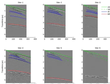
Figure 3. Wide-angle radar data showing air waves (AW, green lines) and surface waves (SW, green dashed lines) with linearly increasing
traveltime with offset, while traveltime increases hyperbolically with offset for internal (blue) and basal (red) reflectors. See Fig. 2 for locations of Sites 1–6. Site 6 was excluded from further analysis because the basal reflection is ambiguous (probably due to off-angle reflectors in the vicinity).
The maximum amplitude of the basal reflector was detected automatically and shifted with a constant offset to the first break. Internal reflectors were handpicked. Figure 3 shows radargrams collected at all sites with the picked reflectors that were used for the analysis. The maximum offset for each site was chosen to equal approximately the local ice thick-ness. At Site 6, basal and internal reflectors are overlaid with signals from off-angle reflectors and cannot be picked unam-biguously. We present the data here to exemplify a case for which WARR does not yield reliable results and exclude this site from further analysis.
2.2 Model parameterization and linearization
The traveltimetNr,No of a ray reflected from a reflectorNr (r∈ [1, R]) at depthDrmeasured at offsetNo(o∈ [1,0]) is given by a line integral over the inverse of the radio-wave ve-locityvalong the ray pathL(extending from the transmitter to the receiver via the reflection boundary).
tNr,No=
Z
L(mv,Dr)
1
v (mv)
dl. (1)
Figure 1 illustrates the notation. For each site, we pick a num-ber of reflectors at different depthsmD=(D1, . . ., DR)T, and
we parameterize the velocity function as a function of density using the model parametersmv. We use an inverse method to reconstruct both the reflector depths and the velocity profile from the measured traveltimes.
The traveltime is a non-linear function of the model pa-rameters (and hence the inversion results may be non-unique) becauseLdepends both on the initially unknown radio-wave propagation speed and the reflector depth. The velocity be-tween two radar reflectors is often represented as piecewise constant or piecewise linear (Brown et al., 2012), making the model parametersmveither the interval velocities or the interval velocity gradients, respectively. Here, we introduce additional constraints from Hubbard et al. (2013) who fit a depth profile of density of the form:
ρ=910−Ae−rz (2)
to density measurements of the borehole recovered at RBIS in 2010. The parametersAandr are tuning parameters for the surface density and the densification length, respectively. We relate density to the radio-wave propagation speedv us-ing the complex refractive index method (CRIM) equation (Wharton et al., 1980; Brown et al., 2012):
ρ=cv
−1−1
wherevi=168 m µs−1is the radio-wave propagation speed in pure ice andcis the speed of light in a vacuum.
Combining Eqs. (2) and (3) leads to
v(A, r)= c
kρ(A, r)+1, (4)
withk= 1 ρi
c vi −1
andmv=(A, r)T. We use Eq. (4) and assume that (i) radio-wave propagation speedvdepends only on density (i.e., excluding ice anisotropy); (ii) density is hor-izontally homogeneous over the maximum lateral offset of the receiver (≤404 m) but varies with depth so thatv only varies with depth in that interval; and (iii) within this inter-val, internal reflectors are horizontal. We aim to detect lat-eral variations of the velocity profiles on larger scales (i.e., between Sites 1 and 5) by finding optimal sets of parame-tersm=(mD,mv)=(A, r, D1, . . ., DR)T ∈RNm describing the data at each site. The number of model parametersNm= R+2 depends on the number of reflectors.
Using Eq. (4) and approximating the integral through a summation overNzdepth intervals, Eq. (1) reads
tNr,No(m)≈
1
c
Nz
X
i=1
lzi(m) (kρ (mv)+1) . (5)
The problem is linearized using an initial guess (marked with superscript 0) and a first-order Taylor expansion:
tNr,No(m)≈t
0
Nr,No+ Nm
X
j=1 ∂tNr,No
∂mj
m0j
mj−m0j
. (6)
An equation of type (6) holds for allO offsets of allR re-flectors and can be summarized in matrix notation:
ε=S1m, (7)
where we defineε=tmod−tobs∈RNpas a vector composed of the residuals between the observed (tobs) and the mod-eled (tmod) traveltimes.Npis the total number of picked dat-apoints for all reflectors (not all reflectors can be picked to the maximum offset O), S∈RNp×Nm is a matrix contain-ing all partial derivatives, and 1m∈RNm is the model up-date vector. One synthesized reflector is composed of more than 50 independent measurements and at each site R=4 re-flectors (including the basal reflector) were picked. There are therefore six model parameters (Nm=4+2 for four reflec-tor depths and two parametersAandrdescribing the depth– density function) and the number of measurements (Np) is typically larger than 200, turning Eq. (7) into an overdeter-mined system of equations.
The derivatives of Eq. (6) with respect toAandrare
∂tNr,No
∂A = −
k c
Nz
X
i=1 lzie
−rzi (8)
∂tNr,No
∂r =
Ak c
Nz
X
i=1
zilzie−rzi, (9)
and ∂tNr,No
∂Dn (n∈ [1, R]) follows from geometric
considera-tions (Zelt and Smith, 1992):
∂tNr,No
∂Dn
=2cos2Nr,No
v(Dn)
δnr, (10)
where2Dn,Nois the incidence angle of rayNoat the reflector boundaryNr=n(Fig. 1b);δnr=1 forr=nand 0 otherwise. An optimal set of model parametersmis found as follows. (i) Starting with an initial estimate for the reflector depths mD0and the velocity modelmv0, a ray tracing forward model
(Sect. 2.3) calculates the expected traveltimes tNr,No0 for a given set of transmitter–receiver offsets; the difference be-tween modeled and observed traveltimes results in the misfit vectorεin Eq. (7). (ii) The overdetermined system is inverted for the unknown parameter-correction vector1m(Sect. 2.4), and (iii) the parameter set is updated withm1=m0+1m and serves as new input for the forward model. These steps are repeated iteratively until the parameter updates are negli-gible.
2.3 Ray tracing forward model
We apply the ray tracing model provided by Margrave (2011) only to reflected (and not to refracted) rays. For a given set of reflectors in av(z)medium, no analytical solution exists which directly provides a ray path from the transmitter to a given offset via a reflection boundary. The problem is solved iteratively by calculating fans of rays with varying take-off angles until one ray endpoint emerges within a given mini-mum distance (≤0.5 m) to the receiver. For somev(z) con-figurations no such ray can be found, indicating that the pre-scribedv(z)medium does not adequately reproduce the ob-servations.
2.4 Inversion
To solve the inverse problem we seek the set of parameters mthat minimizes the cost functionJ:
J=1
2ε
TC−1 t ε+
1 2λ
m−m0TCm−1m−m0, (11) in which the first term is the`2norm of the traveltime resid-ual vector weighted with Ct=diag{σi2}, whereσiis the un-certainty of the traveltime picks. The second term is a regu-larization (weighted with Cm=diag{σj2}, whereσjis the
with the Lagrange multiplier λ is needed because outliers in the data are weighted disproportionally in a least-squares sense, which can lead to overfitting the data.
We minimizeJby updatingmiteratively according to the Gauss–Newton method:
mi+1=mi−STC−t 1S+λC−m1 −1
∇J, (12)
with∇J=C−t 1Sε+λC−m1 m−m0. High values ofλresult in a final model vector remaining close to the initial guess; lower values ofλallow for larger changes in the parameter updates. We stop iterating when changes inJ are below an arbitrarily small threshold.
2.5 Sensitivity of the firn-air content
In order to compare different measurements at different loca-tions, we decompose the ice shelf into two layers of ice (Hi) and air (HA) so thatρH¯ =ρiHi+ρaHA andHi+Ha=H (i.e.,HA=ρaρ¯−−ρiρiH). The firn-air contentHA (with air
den-sityρa) is a quantity independent of the local ice thickness (as long as the depth-averaged radio-wave speed is determined below the firn–ice transition) and changes thereof indicate changes in the depth-averaged density due to a changing firn-layer thickness. The firn-air content in Antarctica can vary from HA=0 m in blue ice areas up toHA=45 m for cold firn on the Antarctic plateau (Ligtenberg et al., 2014). Using the CRIM equation to determineHAresults in
HA= cH ρi
1 ¯
v−
1
vi
(ρa−ρi)
c vi −1
. (13)
We consider errors in HA from uncertainties in the depth-averaged radio-wave propagation speed (v¯), and uncertain-ties in ice thickness (H):
δHA2≈
cρi
v2(ρa−ρi)c vi−1
H δv¯
2
+
cρi
1
¯
v−
1 vi
(ρa−ρi)
c vi−1
δH
2
.
(14) Assumingδv¯≈1 %, andδH≈10 % renders the first term of Eq. (14) about 8 times larger than the second for the parame-ter ranges considered here, and we therefore neglect errors in ice thickness for the error propagation. Equation (14) shows that the uncertainty ofHAscales with the local ice thickness so that small errors in the depth-averaged velocities (<1 %) result in significant errors in terms ofHA. We useHA as a sensitive metric, both for comparing sites laterally and illus-trating uncertainties of the radar method. In the following, we use synthetic data to choose optimal parameters for the inversion, and to investigate how errors in the data propagate into the final depth–density estimates.
2.6 Testing with synthetic examples
To test the inversion algorithm we use ray tracing with a prescribed depth–density function and recording geometry (A=460 kg m−3, r=0.033 m−1; transmitter–receiver off-sets between 30 and 300 m with 2 m spacing) to create a syn-thetic traveltime data set with multiple reflectors. We first in-vestigate whether the solution is well constrained for ideal cases, and then we discuss effects of systematic and random errors in the data.
We consider two ideal cases: a single reflector at 400 m depth, and two reflectors at 30 and 400 m depth. Using the forward model, we simulated a new set of reflectors with model parameters covering depth ranges of±5 m from the ideal depths and depth–density functions defined by r=
0.01−0.1 m−1(Awas fixed). This density range corresponds to firn-air contents from HA=5 to 50 m. The root-mean-square differences (1trms) between the perturbed and the ideal reflector are equivalent to the first term of the objective functionJ (Eq. 11) and indicate how well constrained the solution is. Figure 4a illustrates that for a single reflector the solution is not well constrained, meaning that different sets of model parameters give similar results to the ideal solution (i.e., dense firn/shallower reflector or less dense firn/deeper reflector). For example, positioning the reflector at 392 m depth with r=0.063 m−1 results in a firn-air content of
∼11 m, whereas positioning the reflector at 410 m depth with
r=0.014 m−1corresponds to a firn-air content of approxi-mately 40 m. Both cases have a small model–data discrep-ancy and are barely distinguishable from the ideal solution. Using two reflectors simultaneously better constrains the so-lution, particularly if the shallower reflector is above the firn– ice transition (Fig. 4b). We conclude from these simple test cases that using the basal reflector alone is inadequate. In-stead, multiple reflectors should be considered and inverted for simultaneously. Using this type of testing, we also find (i) that treatingAas a free parameter introduces significant tradeoffs with r even for small noise levels. We therefore keepA fixed and assume in the following that the surface density is laterally uniform; (ii) plotting both terms of the objective functionJ (Eq. 11) versus each other for differ-entλ(a.k.a. L-curve) helps to choose an optimalλ. We find thatλ≈0.1 marks approximately the kink point between too large a model–data discrepancy on the one hand and overfit-ting on the other hand. We keepλ=0.1 from hereon to pre-vent overfitting, but note that results are largely independent ofλforλ0.1.
differ-Reflector depth 1 (m)
Densification length (r, m
−1) (a)
390 395 400 405 410
0.01
0.02
0.03
0.04
0.05
0.06
∆
trms
(
µ
s)
0 0.005 0.01 0.015 0.02
25 28
30 32
0 0.05 0.1 395 400 405
Reflector depth 1 (m)
Densification length (r, m
−1
)
Reflector Depth 2 (m)
(b)
∆
trms
(
µ
s)
0 1 2 3 4 5
x 10−3
Figure 4. Traveltime residuals (1trms) calculated with ray tracing between ideal reflector in a fixed depth–density profile (A=460 kg m−3;
r=0.033 m−1) with reflectors perturbed in terms of depths and density. Ideal solutions are marked with red crosses: (a) traveltime residuals for an ideal reflector at 400 m depth; (b) volumetric slice plot of traveltime residuals for two idealized reflectors at 30 and 400 m depth.
0 200 400 0.5
1 1.5 2 2.5 3 3.5 4
Offset (m)
Traveltime (
µ
s)
Initial estimate (r=0.05 m−1) (a)
Data Model Model at control
0 200 400 0.5
1 1.5 2 2.5 3 3.5 4
Offset (m)
Traveltime (
µ
s)
Final estimate (r=0.027 m−1) (b)
0 200 400 −0.02
0 0.02 0.04 0.06 0.08
Offset (m)
Traveltime residual (
µ
s)
Data−model misfit (c)
Initial estimate Final estimate Initial control Final control
Figure 5. Example for initial (a) and final (b) fit between the ray tracing forward model and the reflectors at Site 2. In this case, three
reflectors (black dots) were used for the inversion and one reflector was kept for control. The forward model corresponds to the red dashed curves and the control reflectors to the blue dashed curves. Initial estimates shown here werer0=0.05 m−1,D1=68.2 m,D3=112.9 m,
D4=291.2 m; the best fit resulted inr=0.027 m−1,D1=67.7 m,D3=111.2 m, andD4=293.3 m. The traveltime residual between the model and data for initial (x) and final fit (o) is shown in (c).
ent magnitudes of noise and systematic errors. We find that the limiting factor for the initial depth guess is the forward model which does not find ray paths for all offsets if the ini-tial guess is further than∼15 m from the true solution. For all initial guesses deviating less than that, the inversion re-covers the true depths robustly within decimeters, even for noise levels with a mean amplitude of 5 times the sampling interval (0.01 µs). However, the inversion is most sensitive to trends in the data. For example, if reflectors deviate systemat-ically from 0.04 to−0.04 µs for large offsets, reflector depths are reconstructed with an error of 2–3 m. The corresponding densities deviate in terms of firn-air content more than 5 m from the ideal solutions. We conclude from these test cases that reflectors need to be picked accurately (i.e keeping the same phase within the individual wavelets); if systematic dif-ferences between the forward model and data occur (e.g., the modeled reflector is tilted with respect to the observations), then results should be interpreted with care.
2.7 Inversion of field data
For each site, three internal reflectors were handpicked (D1– D3) to complement the automatically detected basal reflec-tor (D4, Fig. 3). Initial guesses for reflector depths are based on standard linear regression in the traveltime2–offset2 di-agrams (Dix, 1955); r0=0.033 m−1 and A=460 kg m−3 stem from the 2010 OPTV density profile (Hubbard et al., 2013).
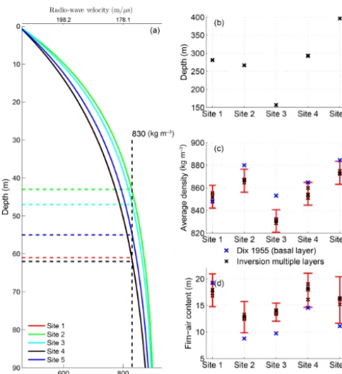
Figure 6. Derived data summary of all sites (Site 3 is located in
an ice-shelf channel): (a) depth–density profiles inverted from four reflectors, (b) ice thickness, (c) depth-averaged density, and (d) firn-air content. Black crosses in (b–d) represent the outcomes for five combinations containing three or more reflectors. Error bars assume a 1 % error in depth-averaged radio-wave propagation speed. The blue crosses correspond to depth-averaged solutions using normal moveout of the basal reflector only (Dix, 1955).
In a second step, we inverted for all five remaining re-flector combinations containing three and four rere-flectors. We also considered a range forr0between 0.021 and 0.056 m−1, corresponding to a firn-air content of 24 and 9 m, respec-tively. Figure 5 illustrates an example where three reflectors were used for the inversion and one was left for validation; the model–data discrepancy is large for the initial guess. Af-ter the inversion, the model–data discrepancy is smaller for all reflectors including the reflector that was used for control only.
In general, the final results are more sensitive to the respec-tive reflector combination than to the initial guess ofr0. For the latter we chose the one resulting in the smallest model– data discrepancy (r0=0.033 m−1). Differences between the final five parameter sets give a lower boundary for an error estimate.
3 Density from optical televiewing
Densities were evaluated independently from the radar anal-yses using OPTV logs of two boreholes drilled in 2010 and 2014 (Fig. 2). OPTV exploits the density dependence
Figure 7. Depth profiles of density derived from WARR (dashed)
and OPTV (solid). WARR data are from Sites 1 and 3, closest to the OPTV sites. Site 3 and the 2014 borehole are both in the trough of an ice-shelf channel (Fig. 2). The envelopes of the radar-derived densities correspond to the lower and upper limit of five reflector combinations used for the inversion. The OPTV logs were smoothed with a 0.5 m running mean.
of backscattered light within the borehole. By lowering an OPTV device into boreholes, luminosity (i.e., density) pro-files can be collected with a vertical resolution of millimeters (Hubbard et al., 2008). This has been demonstrated for the 2010 borehole at RBIS (Hubbard et al., 2013) and we re-fer to this rere-ference for further details on the method. Both borehole OPTV logs were calibrated against at least 40 den-sity measurements made directly on core samples, yielding anR2value between luminosity and density of 0.96 for the 2010 log (Hubbard et al., 2013) and 0.82 for the 2014 log.
4 Results
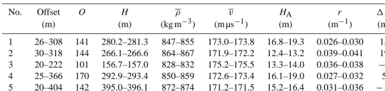
re-Table 1. Summary of the WARR results from sites 1–5 in terms of range of offsets, number of offsets (O), ice thickness (H), depth-averaged density (ρ), depth-averaged radio-wave propagation speed (v), firn-air content (HA), the decay length (r) parameterizing the depth– density function, and the deviation from hydrostatic equilibrium (1H). The ranges correspond to the lower and upper limits of five reflector combinations at each site (four reflector combinations contain three reflectors, and one combination contains all four reflectors).
No. Offset O H ρ v HA r 1H
(m) (m) (kg m−3) (m µs−1) (m) (m−1) (m)
1 26–308 141 280.2–281.3 847–855 173.0–173.8 16.8–19.3 0.026–0.030 15 2 30–318 144 266.1–266.6 864–867 171.9–172.2 12.4–13.2 0.039–0.041 19 3 20–222 101 156.7–157.0 828–832 175.2–175.5 13.3–14.0 0.036–0.038 −4 4 25–366 170 292.9–293.4 850–859 172.6–173.4 16.1–19.0 0.027–0.032 5 5 20–404 142 395.0–396.1 872–874 171.2–171.5 15.2–16.4 0.031–0.036 −13
sults are numerically robust to the combination of reflectors used, and that the local ice thickness and depth-averaged den-sity can be determined with high confidence. However, we cannot derive rigorous error estimates from the inversion it-self. We found that picking the internal reflectors is the most sensitive step and, similar to Brown et al. (2012), we es-timate that the depth-averaged velocity can be determined within ±1 %. We used this value to calculate errors for the depth-averaged densities and the equivalent firn-air content. These errors roughly take into account the assumptions of non-dipping reflectors, ice isotropy, and uncertainties of the density–permittivity model.
The estimated 1 % error on the (depth-averaged) radio-wave propagation speed translates into large error bars for the corresponding firn-air contents (Fig. 6d), impeding the comparison between sites. Nevertheless, Sites 2 and 3 show lower firn-air contents (∼13 m) than the other sites (∼17 m). To assess the derived depth–density profiles with an in-dependent data set, we compare Site 1 and Site 3 with the OPTV densities from the 2010 and 2014 boreholes, respec-tively (Fig. 7). Site 3 is located inside an ice-shelf channel, about 10 km north of the 2014 borehole located in the same channel. Site 1 is about 6 km south of the 2010 borehole (Fig. 2). Both radar WARR measurements and the OPTV logs show a depth–density profile that is denser inside than outside the ice-shelf channel. This increases our confidence that the WARR method developed here indeed picks up sig-nificant differences in firn-air content on small spatial scales.
5 Discussion
5.1 Benefits of traveltime inversion using ray tracing A difference between the new study presented here and pre-vious ones (e.g., Brown et al., 2012) is how the radio-wave propagation speed is parameterized. Previous studies used piecewise linear or uniform speed between individual reflec-tors, while we parameterize the speed as a continuous func-tion of depth (Eq. 4). Here, we examine the benefit of this approach for interpreting the radar results
A common problem when using the Dix inversion or sem-blance analysis is that the applied normal moveout (NMO) approximation presupposes small reflection angles (to lin-earize trigonometric functions) and small velocity contrasts (Dix, 1955). In our case reflection angles can be large (<45◦), particularly near the maximum offsets; contrary to NMO, ray tracing is not adversely influenced by wide in-cidence angles. NMO presupposes small velocity contrasts, because ray paths are approximated as oblique lines ne-glecting raybending from a gradually changing background medium. Traveltime inversion with ray tracing equally re-lies on this approximation as long as interval velocities are assumed. In this study, we prescribe a realistic shape of a depth–density/velocity function, which changes gradually with depth, and raybending is taken into account adequately during the ray tracing. We have tested both the small angle and the small velocity contrast limitations quantitatively by using the OPTV-based depth–density/velocity function and ray tracing in order to simulate synthetic traveltimes of re-flectors at various depths (50–500 m) and horizontal offsets (50–500 m). We then used the synthetic traveltimes for calcu-lating the reflector depths and the depth-averaged velocities (averaged from the surface to the reflector depths) subject to the NMO equations. Differences in depth-averaged velocities were smaller than 0.5 %, and differences in reflector depths were smaller than 0.5 m. Similar to the findings of Barrett et al. (2007), this confirms that in our case the NMO approx-imation essentially holds, even for comparatively large hor-izontal offsets and a continuously changing depth–velocity function. This must not always be the case and ray tracing easily allows the NMO approximation to be checked for each specific setting. For the examples considered here, solutions based on the Dix inversion, using only the basal reflector, typically result in thicker ice and higher depth-averaged den-sities (and correspondingly lower firn-air contents, Fig. 6c– d).
1987). The choice for the acquisition geometry thus depends on the time available in the field and on the glaciological setting (i.e., whether dipping reflectors are to be expected). Traveltime inversion can cope with both types of acquisi-tion geometries. If reflector dips are important, the routine presented here can be adapted to include one dip angle per reflector in the inversion. However, given that including the surface density as an additional free parameter is difficult if all parameters are inverted simultaneously, an iterative ap-proach may be required to find one depth–density function for all reflectors while solving for the reflector dips individu-ally (layer stripping; Brown et al., 2012).
The main advantages of the method applied here are pri-marily linked to a more robust inversion, which is less sentive to reflector delineation because reflectors are inverted si-multaneously to constrain the density profile. First, prescrib-ing a global depth–density/velocity function for all internal reflectors allows the coherency of the reflector picking to be checked by investigating different subsets of reflector com-bination to single out reflectors, which were picked with the wrong phase (Sect. 2.7). This step is important, particularly when using lower frequencies as was the case here (10 MHz). At this stage the basal reflector is useful, because it can be identified unambiguously. Once more than two shallow inter-nal reflectors are reliably picked, we found that the inversion results were largely independent of the inclusion of the basal reflector. Second, by inverting for reflectors simultaneously, it is less likely that deeper reflectors inherit uncertainties from shallower reflectors. This can happen when solving for reflectors individually where tradeoffs between interval ve-locities and reflector depths are subsequently handed down-wards. Third, when using interval velocities, the parameter set describing the depth–density/velocity function is larger than is the case here. For example, for four reflectors eight parameters are required when using interval velocities (four velocities and reflector depths, respectively), and this com-pares with only the five parameters that we required for the method applied here (r and four reflector depths). Simpler models with fewer model parameters are preferable when us-ing inversion.
Based on our synthetic examples, we found that the travel-time inversion used here is unstable if all parameters (sur-face density, densification length, reflector depths) are in-verted for simultaneously. We therefore considered the sur-face density to be laterally uniform, which is not supported by empirical data. In principle, the surface density can be es-timated from the data by picking the linear moveout of the surface wave (green dashed lines in Fig. 3, cf. Brown et al., 2012). However, in our 10 MHz data set the surface wave cannot be identified unambiguously, resulting in a large range of possible surface densities. We addressed this point with a sensitivity analysis including a range of surface densities (300≤A≤500 kg m−3). The smallest model–data discrep-ancies are found with A≈400 kg m−3, but in all cases the final results do not deviate more than the error bars provided
in Fig. 6. This means that the ill-constrained surface density is essentially corrected for during the inversion by adapting the densification length.
The WARR data presented here were collected with a 10 MHz radar. The disadvantage of this low frequency is that fewer reflectors above the firn–ice transition can be picked at this low resolution, relative to higher-frequency data sets (cf. Eisen et al., 2002 who derived an 8 % velocity error with a 25 MHz radar versus a 2 % error with 200 MHz radar). We found that the method applied here can cope with the picking uncertainties at 10 MHz, whereas using Dix inversion fre-quently resulted in interval densities much larger than the pure ice density. The advantage of using a 10 MHz radar is that the entire ice column is illuminated, including the un-ambiguous basal reflector. This opens up the possibility for more sophisticated radar-wave velocity models including ice anisotropy originating from aligned crystal orientation fab-ric below the firn–ice transition (Drews et al., 2012; Mat-suoka et al., 2012b). The radar data set is also suited for other glaciological applications, for example, using the basal re-flections for deriving ice temperature (via radar attenuation rates) from an amplitude versus offset analysis (Winebrenner et al., 2003) and constraining the alignment of ice crystals us-ing multistatic radar as a large-scale Rigsby stage (Matsuoka et al., 2009).
5.2 Radar- and OPTV-inferred densities
We found velocity models for each site which adequately fit all reflector combinations. There is no systematic deviation larger than the picking uncertainty and hence there is no ev-idence that reflectors dip within the interval between mini-mum and maximini-mum offset (≤404 m). The results are numer-ically robust for different reflector combinations, indicating equal validity for all results based on three reflectors or more (Sect. 2.7).
The derived depth–density functions cluster into two groups: Sites 1, 4, and 5 have a mean firn-air content of
good fit is found between Site 3 and the 2014 OPTV (both located inside the same ice-shelf channel, Fig. 7). The im-plications are twofold: first, the correspondence between the OPTV-derived density variations and those derived from the WARR method provides independent validation of the lat-ter technique. Second, the fact that both techniques show in-creased density within the surface channel indicates that the effect is real and should be accounted for by investigations based on hydrostatic equilibrium. However, given that Site 2 also shows a comparatively low firn-air content, we cannot unambiguously conclude from the data alone that firn den-sity is elevated in ice-shelf channels in general. One potential mechanism for such a behavior is the collection of meltwater in the channel’s surface depressions. At RBIS, surface melt can be abundant in the (austral) summer months, particularly in an about 20 km wide blue ice belt near the grounding line. The most recent Belgian Antarctic Research Expedition (Jan-uary 2016) observed frequent melt ponding and refreezing in this area, mostly in the vicinity of ice-shelf channels where meltwater preferentially collects in the small-scale surface depressions. If this holds true, the increased density observed in the WARR data close to the ice-shelf front is an inherited feature from farther upstream. The channel’s surface depres-sions likely also cause a locally increased surface mass bal-ance (Langley et al., 2014), and in general ice-shelf chan-nels can have a particular strain regime (Drews et al., 2015). Both of these factors may also influence the firn densification rate, but given our limited data coverage we refrain from an in-depth analysis here. More work is required to determine whether firn in ice-shelf channels is systematically denser.
Even though uncertainties remain about what causes the density variations, we have shown that traveltime inversion and ray tracing with a prescribed shape for the depth–density function can produce results, which compare closely with densities derived from OPTV (excluding small-scale vari-ability due to melt layers). The data presented here show that a lateral density variability requires attention, particu-larly when using mass conservation to derive basal melt rates in ice-shelf channels. Errors in the firn-air content propagate approximately with a factor of 10 into the hydrostatic ice thickness, which then substantially alters the magnitude of derived basal melt rates. Using the same parameters as Drews et al. (2015), we compare the WARR-derived ice thickness with the hydrostatic ice thickness for each site. We find a maximum deviation of 19 m for Site 2, and a minimum de-viation of 4 m for Site 3 (Table 1). Assuming the absence of marine ice, those deviations are comparatively small given the uncertainties of the geoid and the mean dynamic topog-raphy, both of which are required parameters for the hydro-static inversion.
6 Conclusions
We have collected six wide-angle radar measurements on RBIS and used traveltime inversion in conjunction with ray tracing to infer the local depth–density profiles. In the in-version, we prescribed a physically motivated shape for the depth–density function, which adequately takes curved ray paths and large reflection angles into account and allows the simultaneous inversion of multiple reflectors. We find that this method produces robust results, even with a com-paratively low-frequency (10 MHz) radar system with cor-respondingly reduced spatial resolution and small numbers of internal reflectors used to constrain the density model. The inversion method is flexible and can be adapted to other acquisition geometries and radar frequencies. Ice thickness and depth-averaged densities/wave speed are reconstructed within a few percent. Larger errors in the corresponding firn-air contents, however, impede detailed comparison between sites. Nevertheless, spatial variations in densities derived from both wide-angle radar and borehole optical teleview-ing show that se-2015-112the depth–density profile within a 2 km wide ice-shelf channel is denser inside than outside that channel. This density anomaly needs to be accounted for when using hydrostatic equilibrium to infer ice thickness, and has implications for using mass budget methods to de-termine basal melting in ice-shelf channels. More data are needed to evaluate whether the density anomaly observed here is a generic feature of ice-shelf channels in Antarctica.
Acknowledgements. This paper forms a contribution to the Belgian
Research Programme on the Antarctic (Belgian Federal Science Policy Office), project SD/SA/06A “Constraining ice mass changes in Antarctica” (IceCon), as well as the FNRS-FRFC (Fonds de la Recherche Scientifique) project IDyRA. We thank the InBev Baillet Latour Antarctica Fellowship for financing the RBIS fieldwork and the International Polar Foundation for providing all required logis-tics in the field. We thank in particular A. Hubert, K. Moerman, K. Soete, and L. Favier for support in the field. Morgane Philippe is partially funded through a grant from the “Fonds David et Alice Van Buuren”. The comments of two reviewers and the editor R. Bingham have improved the initial version of this manuscript. A version of the code is accessible on request and on GitHub (https://github.com/rdrews/).
Edited by: R. Bingham
References
Arthern, R. J., Vaughan, D. G., Rankin, A. M., Mulvaney, R., and Thomas, E. R.: In situ measurements of Antarctic snow com-paction compared with predictions of models, J. Geophys. Res., 115, F03011, doi:10.1029/2009jf001306, 2010.
using a stepped-frequency radar, J. Geophys. Res.-Earth, 118, 1257–1263, doi:10.1002/jgrf.20089, 2013.
Barrett, E. B., Murray, T., and Clark, R.: Errors in Radar CMP Ve-locity Estimates Due to Survey Geometry, and Their Implication for Ice Water Content Estimation, J. Environ. Eng. Geoph., 12, 101–111, doi:10.2113/JEEG12.1.101, 2007.
Bender, M., Sowers, T., and Brook, E.: Gases in ice cores, P. Natl. Acad. Sci. USA, 94, 8343–8349, doi:10.1073/pnas.94.16.8343, 1997.
Blindow, N., Suckro, S. K., Rückamp, M., Braun, M., Schindler, M., Breuer, B., Saurer, H., Simões, J. C., and Lange, M. A.: Ge-ometry and thermal regime of the King George Island ice cap, Antarctica, from GPR and GPS, Ann. Glaciol., 51, 103–109, doi:10.3189/172756410791392691, 2010.
Booth, A., Clark, R., and Murray, T.: Semblance response to a ground-penetrating radar wavelet and resulting errors in veloc-ity analysis, Near Surf. Geophys., 8, 235–246, doi:10.3997/1873-0604.2011019, 2010.
Booth, A., Clark, R., and Murray, T.: Influences on the resolution of GPR velocity analyses and a Monte Carlo simulation for es-tablishing velocity precision, Near Surf. Geophys., 9, 399–411, doi:10.3997/1873-0604.2011019, 2011.
Bradford, J. H., Harper, J. T., and Brown, J.: Complex dielectric permittivity measurements from ground-penetrating radar data to estimate snow liquid water content in the pendular regime, Water Resour. Res., 45, W08403, doi:10.1029/2008WR007341, 2009. Brown, J., Bradford, J., Harper, J., Pfeffer, W. T., Humphrey, N., and
Mosley-Thompson, E.: Georadar-derived estimates of firn den-sity in the percolation zone, western Greenland ice sheet, J. Geo-phys. Res., 117, F01011, doi:10.1029/2011JF002089, F01011, 2012.
Cuffey, K. and Paterson, W.: The physics of Glaciers, 4th Edn., Burlington, MA, Academic Press, 2010.
Depoorter, M. A., Bamber, J. L., Griggs, J. A., Lenaerts, J. T. M., Ligtenberg, S. R. M., van den Broeke, M. R., and Moholdt, G.: Calving fluxes and basal melt rates of Antarctic ice shelves, Na-ture, 502, 89–92, doi:10.1038/nature12567, 2013.
Dix, C. H.: Seismic Velocities from Surface Measurements, Geo-physics, 20, 68–86, doi:10.1190/1.1438126, 1955.
Drews, R.: Evolution of ice-shelf channels in Antarctic ice shelves, The Cryosphere, 9, 1169–1181, doi:10.5194/tc-9-1169-2015, 2015.
Drews, R., Eisen, O., Steinhage, D., Weikusat, I., Kipfstuhl, S., and Wilhelms, F.: Potential mechanisms for anisotropy in ice-penetrating radar data, J. Glaciol., 58, 613–624, doi:10.3189/2012JoG11J114, 2012.
Drews, R., Matsuoka, K., Martín, C., Callens, D., Bergeot, N., and Pattyn, F.: Evolution of Derwael Ice Rise in Dronning Maud Land, Antarctica, over the last millennia, J. Geophys. Res.-Earth, 120, 564–579, doi:10.1002/2014JF003246, 2015.
Dutrieux, P., Vaughan, D. G., Corr, H. F. J., Jenkins, A., Holland, P. R., Joughin, I., and Fleming, A. H.: Pine Island glacier ice shelf melt distributed at kilometre scales, The Cryosphere, 7, 1543– 1555, doi:10.5194/tc-7-1543-2013, 2013.
Eisen, O., Nixdorf, U., Wilhelms, F., and Miller, H.: Elec-tromagnetic wave speed in polar ice: validation of the common-midpoint technique with high-resolution dielectric-profiling and -density measurements, Ann. Glaciol., 34, 150– 156, doi:10.3189/172756402781817509, 2002.
Eisen, O., Frezzotti, M., Genthon, C., Isaksson, E., Magand, O., van den Broeke, M. R., Dixon, D. A., Ekaykin, A., Holm-lund, P., Kameda, T., Karlöf, L., Kaspari, S., Lipenkov, V. Y., Oerter, H., Takahashi, S., and Vaughan, D. G.: Ground-based measurements of spatial and temporal variability of snow ac-cumulation in East Antarctica, Rev. Geophys., 46, RG2001, doi:10.1029/2006RG000218, 2008.
Freitag, J., Kipfstuhl, S., and Laepple, T.: Core-scale radioscopic imaging: a new method reveals density–calcium link in Antarc-tic firn, J. Glaciol., 59, 1009–1014, doi:10.3189/2013JoG13J028, 2013a.
Freitag, J., Kipfstuhl, S., Laepple, T., and Wilhelms, F.: Impurity-controlled densification: a new model for stratified polar firn, J. Glaciol., 59, 1163–1169, doi:10.3189/2013JoG13J042, 2013b. Gladish, C. V., Holland, D. M., Holland, P. R., and Price, S. F.: Ice-shelf basal channels in a coupled ice/ocean model, J. Glaciol., 58, 1227–1244, doi:10.3189/2012JoG12J003, 2012.
Gregory, S. A., Albert, M. R., and Baker, I.: Impact of physical properties and accumulation rate on pore close-off in layered firn, The Cryosphere, 8, 91–105, doi:10.5194/tc-8-91-2014, 2014. Griggs, J. and Bamber, J.: Antarctic ice-shelf thickness
from satellite radar altimetry, J. Glaciol., 57, 485–498, doi:10.3189/002214311796905659, 2011.
Hempel, L., Thyssen, F., Gundestrup, N., Clausen, H. B., and Miller, H.: A comparison of radio-echo sounding data and elec-trical conductivity of the GRIP ice core, J. Glaciol., 46, 369–374, doi:10.3189/172756500781833070, 2000.
Herron, M. M. and Langway, C. C.: Firn Densification: An empiri-cal Model, J. Glaciol., 25, 373–385, 1980.
Hörhold, M. W., Kipfstuhl, S., Wilhelms, F., Freitag, J., and Frenzel, A.: The densification of layered polar firn, J. Geophys. Res., 116, F01001, doi:10.1029/2009JF001630, 2011.
Hörhold, M. W., Laepple, T., Freitag, J., Bigler, M., Fischer, H., and Kipfstuhl, S.: On the impact of impurities on the densi-fication of polar firn, Earth Planet. Sc. Lett., 325-32, 93–99, doi:10.1016/j.epsl.2011.12.022, 2012.
Hubbard, B. and Glasser, N.: Field Techniques in Glaciology and Glacial Geomorphology, John Wiley & Sons Ltd., The Atrium, Southern Gate, Chichester, West Sussex, 2005.
Hubbard, B., Roberson, S., Samyn, D., and Merton-Lyn, D.: Digital optical televiewing of ice boreholes, J. Glaciol., 54, 823–830, doi:10.3189/002214308787779988, 2008.
Hubbard, B., Tison, J.-L., Philippe, M., Heene, B., Pattyn, F., Mal-one, T., and Freitag, J.: Ice shelf density reconstructed from opti-cal televiewer borehole logging, Geophys. Res. Lett., 40, 5882– 5887, doi:10.1002/2013GL058023, 2013.
Kawamura, T.: Nondestructive, three-dimensional den-sity measurements of ice core samples by X ray com-puted tomography, J. Geophys. Res., 95, 12407–12412, doi:10.1029/JB095iB08p12407, 1990.
Kovacs, A., Gow, A. J., and Morey, R. M.: The in-situ dielectric constant of polar firn revisited, Cold Reg. Sci. Technol., 23, 245– 256, doi:10.1016/0165-232X(94)00016-Q, 1995.
Le Brocq, A., Ross, N., Griggs, J., Bingham, R., Corr, H., Fer-raccioli, F., Jenkins, A., Jordan, T., Payne, A., Rippin, D., and Siegert, M.: Evidence from ice shelves for channelized meltwater flow beneath the Antarctic Ice Sheet, Nat. Geosci., 6, 945–948, doi:10.1038/ngeo1977, 2013.
Lenaerts, J. T. M., Brown, J., van den Broeke, M. R., Matsuoka, K., Drews, R., Callens, D., Philippe, M., Gorodetskaya, I. V., van Meijgaard, E., Reijmer, C. H., Pattyn, F., and van Lipzig, N. P. M.: High variability of climate and surface mass bal-ance induced by Antarctic ice rises, J. Glaciol., 60, 1101–1110, doi:10.3189/2014JoG14J040, 2014.
Ligtenberg, S. R. M., Kuipers Munneke, P., and van den Broeke, M. R.: Present and future variations in Antarctic firn air con-tent, The Cryosphere, 8, 1711–1723, doi:10.5194/tc-8-1711-2014, 2014.
Looyenga, H.: Dielectric constants of heterogeneous mixtures, Physica, 31, 401–406, 1965.
Margrave, G. F.: Numerical Methods of Exploration Seismology with algorithms in Matlab, CREWES Toolbox Version: 1006, CREWES Department of Geoscience, University of Calgary, downloaded January 2015, 2011.
Matsuoka, K., Wilen, L., Hurley, S. P., and Raymond, C. F.: Ef-fects of Birefringence Within Ice Sheets on Obliquely Propa-gating Radio Waves, IEEE T. Geosci. Remote, 47, 1429–1443, doi:10.1109/TGRS.2008.2005201, 2009.
Matsuoka, K., Pattyn, F., Callens, D., and Conway, H.: Radar char-acterization of the basal interface across the grounding zone of an ice-rise promontory in East Antarctica, Ann. Glaciol., 53, 29–34, doi:10.3189/2012AoG60A106, 2012a.
Matsuoka, K., Power, D., Fujita, S., and Raymond, C. F.: Rapid de-velopment of anisotropic ice-crystal-alignment fabrics inferred from englacial radar polarimetry, central West Antarctica, J. Geo-phys. Res., 117, F03029, doi:10.1029/2012JF002440, 2012b. Millgate, T., Holland, P. R., Jenkins, A., and Johnson, H. L.: The
ef-fect of basal channels on oceanic ice-shelf melting, J. Geophys. Res.-Oceans, 118, 6951–6964, doi:10.1002/2013JC009402, 2013.
Murray, T., Stuart, G. W., Miller, P. J., Woodward, J., Smith, A. M., Porter, P. R., and Jiskoot, H.: Glacier surge propagation by ther-mal evolution at the bed, J. Geophys. Res., 105, 13491–13507, doi:10.1029/2000JB900066, 2000.
Rignot, E., Jacobs, S., Mouginot, J., and Scheuchl, B.: Ice-Shelf Melting Around Antarctica, Science, 341, 266–270, doi:10.1126/science.1235798, 2013.
Sergienko, O. V.: Basal channels on ice shelves, J. Geophys. Res.-Earth, 118, 1342–1355, doi:10.1002/jgrf.20105, 2013.
Stanton, T. P., Shaw, W. J., Truffer, M., Corr, H. F. J., Peters, L. E., Riverman, K. L., Bindschadler, R., Holland, D. M., and Anan-dakrishnan, S.: Channelized Ice Melting in the Ocean Bound-ary Layer Beneath Pine Island Glacier, Antarctica, Science, 341, 1236–1239, doi:10.1126/science.1239373, 2013.
van den Broeke, M., van den Berg, W. J., and van den Meijgaard, E.: Firn depth correction along the Antarctic grounding line, Antarct. Sci., 20, 513–517, doi:10.1017/S095410200800148X, 2008. Vaughan, D. G., Corr, H. F. J., Bindschadler, R. A., Dutrieux, P.,
Gudmundsson, G. H., Jenkins, A., Newman, T., Vornberger, P., and Wingham, D. J.: Subglacial melt channels and fracture in the floating part of Pine Island Glacier, Antarctica, J. Geophys. Res., 117, F03012, doi:10.1029/2012JF002360, 2012.
Waddington, E. D., Neumann, T. A., Koutnik, M. R., Marshall, H.-P., and Morse, D. L.: Inference of accumulation-rate patterns from deep layers in glaciers and ice sheets, J. Glaciol., 53, 694– 712, doi:10.3189/002214307784409351, 2007.
Wharton, R. B., Rau, R., and Best, D. L.: Electromagnetic propa-gation logging: Advances in technique and interpretation, paper presented at the SPE Annual Technical Conference and Exhi-bition, Dallas, Texas, 21–24 September, doi:10.2118/9267-MS, 1980.
Wilhelms, F., Kipfstuhl, S., Miller, H., Heinloth, K., and Firestone, J.: Precise dielectric profiling of ice cores: A new device with improved guarding and its theory, J. Glaciol., 44, 171–174, 1998. Winebrenner, D. P., Smith, B. E., Catania, G. A., Conway, H. B., and Raymond, C. F.: Radio-frequency attenuation beneath Siple Dome,West Antarctica, from wide-angle and profiling radar observations, Ann. Glaciol., 37, 226–232, doi:10.3189/172756403781815483, 2003.
Wouters, B., Martin-Español, A., Helm, V., Flament, T., van Wessem, J. M., Ligtenberg, S. R. M., van den Broeke, M. R., and Bamber, J. L.: Dynamic thinning of glaciers on the Southern Antarctic Peninsula, Science, 348, 899–903, doi:10.1126/science.aaa5727, 2015.
Yilmaz, O.: Seismic Data Processing, Society of Exploration Geo-physicists, Tulsa, OK, 1987.
Zelt, C. A. and Smith, R. B.: Seismic traveltime inversion for 2-D crustal velocity structure, Geophys. J. Int., 108, 16–34, doi:10.1111/j.1365-246X.1992.tb00836.x, 1992.