© 2016 IJSRST | Volume 2 | Issue 6 | Print ISSN: 2395-6011 | Online ISSN: 2395-602X Themed Section: Science and Technology
Density of Space and Time in the Classical Kinematics of
Material Point
Zvezdelin Ivanov Peykov*, Angel Todorov Apostolov, Nikolai Stamenov Mihailov
Department of Physics, University of Architecture, Civil Engineering and Geodesy, Sofia, Bulgaria
ABSTRACT
The concepts linear differential and average density of space and time have been defined on the ground of the mathematical concept of density of function and arbitrary motion of a material point in its trajectory. An analysis is made of these concepts at various types of motion of material point. It is shown that the density of the space with respect to time at an arbitrary uniform motion is constant in trajectory and is greater than, equal to or less than the density of the time. Its value depends on the magnitude of the velocity of the point. When the motion is variable the density of space with respect to the density of time is not constant. Its value is determined by the magnitude of the tangential acceleration at any point of time.
Keywords :
Density of Space and Time
I.
INTRODUCTION
Let consider the arbitrary motion of a material point in its trajectory. The Law of motion (distance covered):
S = S (t)
represent continuous, differentiable and monotonous function of time, whose exemplary graphic is shown on fig. 1a. (The same applies to the law of the magnitude of the velocity: v = v (t).)
Figure 1: Mutually unique and reversibly compliance between the arrays {St = ct} and {t}
Arrays of values of the argument: {t}, t € [t0, t] and of the function: {S}, S € [S0, S] have a different quality - the first has a dimension of time [s], and the second -
with dimension of length [m]. In order to harmonize their dimensionality we shall choose for argument the array {ct}, where c is the magnitude of some velocity called normalizing velocity (this may not be the velocity of light). Then between the arrays {St = ct} and {t} there is mutually unique and reversibly compliance. The graph of the law S = S(St) takes the type on fig. 1b as on the axes there are equal quality of the function and of the argument - length [m].
We have only to identify c. The normalizing velocity must meet the following conditions:
a) с ≠ 0, с ≠ ∞. Otherwise interval ΔSt = c (t - t0) would be shrunk into a point or would stretch to infinity.
b) c = const – in order the density of the argument {St} to be constant throughout the whole interval ΔSt = cΔt.
c) c should not change the numerical values of the path covered by point:
ΔS(Δt) = ΔS(ΔSt) = ΔS(cΔt)
II.
METHODS AND MATERIAL
A. Definition
In order to define the concepts of density of space and density of time we shall use the following basic postulate:
One material point in its movement on its trajectory at some moment of time t can take only one point of the space.
This postulate provides mutual and unambiguous correlation between each point in space on the trajectory and in any moment of time:
NSi ↔ NSti
Then, using mathematical concept density of function and density of argument [1], we can define the following densities:
1. Density of the Time:
a) Absolute differential linear density:
cdt
dN
dS
dN
Stit Sti t
}
{
}
{
where {dNSti} is the array of values of the argument St in the interval: dSt =cdt.
It is clear that: ρt → ∞ because when dt → 0, {dNSti} → 1. Furthermore, in classical kinematics they supposed that the passage of time in the whole space is uniform. That is why we shall consider that: ρt = const along the entire axis St.
b) Absolute average linear density:
t
c
N
S
N
Stit Sti
t
}
{
}
{
where {NSti} is the array of values of the argument St in the interval: ΔSt = cΔt. Here it is clear as well that:
t
at end interval cΔt.Regarding the connection between the average and differential density of the time we have:
t t
ct
ct t S
S t t t
t ct t c ct d t c dS S
t
t
0 0
) ( 1
2. Density of the Space:
a) Absolute linear differential density:
dS
dN
Sis
}
{
where {dNSi} is the array of values of the function S in the interval: dSt = cΔt.
Analogously here: ρs → ∞ as well, but it is possible the density of the space along the axis S not to be constant: ρs ≠ const.
Of mutual and unambiguous correspondence between the arrays of values of the function and argument {NSi} ↔ {NSti} follows:
t t s
dS
dS
Then:
t t
s
dS
dS
dS
cdt
t t
b) Absolute linear average density:
S
N
Sis
}
{
Here as well:
s
, as
s can be different of ρs. And:t t t t
S
S t t
S
S t t S
S s s
S
t
c
S
ct
ct
dS
S
dS
dS
dS
S
dS
S
)
(
1
1
0
0
0 0
3. Relative linear density of the space in case of one motion of a point to another motion in the identical interval dSt or ΔSt:
S
d
N
d
SiS
{
}
2
,S
d
N
d
SiS
{
}
1
1
12
S
d
S
d
S S
, analogously:
1
12
S
S
S S
4. Relative density of time towards the density of space.
equal density of space:
s
s
const
, we can define the density of time towards the density of space:s s s t t
dS
dS
, s s s
t t
S
S
1
12
t t
t t
S
d
S
d
,
1
12
t t
t t
S
S
All linear densities of space and time introduced here have the equal dimensionalities [1/m].
At so defined density of space a question remains open: what changes in space (time) when its density changes - whether the size of its points or the distance between them?
B. Examination of the density of space in various kinds of motions.
We shall use the theorem of decomposition of a random motion of a material point [2]. We have the law of motion:
tt tdtdttdtdt
t) () () () (r0v0 0 a an r
where
r
(
t
)
is the radius vector of the point in the arbitrary moment of time,
r
0
is the initial radius vector at a moment t0, v0
- initial speed,
a
and
a
n
are respectively tangential and normal acceleration. If we choose the trajectory of the point for summary curvilinear coordinate [3]:S = S(t)
as: S(t0) = S0 , then the law of motion takes the form:
S tt atdtdt
t
S() 0v0( 0)
()where v0 and aτ are algebraic projections of velocity and of tangential acceleration on it. The first two addends:
) ( v0 0
0 t t
S , describe uniform motion on trajectory,
and the third addend:
a(t)dtdt - variable motion without initial velocity. Here, the normal acceleration)
(
t
na
, which defines only the type of the trajectory is not involved (its projection on S is: an(t) = 0 ).Accordingly, the law of velocity has the form:
atdt
t) v () (
v 0
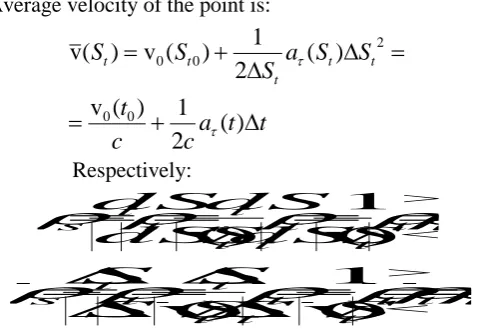
Average velocity of a point on the trajectory is:
t Sv(tt) a(t)dtdt
v 0 0
a
t
dtdt
t
(
)
1
v
v
0 The introduction of normalizing velocity: c = 1 [m / s] in order to equalize the quality of the function and its argument leads to the following changes:
c
t
cdt
dS
dS
dS
S
t t
)
(
v
)
(
v
- dimensionless value;
1
v
(
)
1
(
)
)
(
v
)
v(
)
(
2 2a
t
c
dt
t
d
c
cdt
c
t
d
dS
S
d
S
a
t t
t
with dimensionality [1/m].
Accordingly, the laws for motion and velocity obtain the following form:
dtdt
S
a
c
t
c
S
S
dtdt
c
S
a
S
S
S
S
S
S
t t
t t
t t
t
)
(
)
(
v
)
(
)
(
v
)
(
)
(
2 0
0 0
2 0
0 0 0
with dimensionality [m]
S
a
S
dS
a
S
cdt
S
t t t t(
t)
c
v
)
(
)
(
v
)
v(
00
0
dimensionless value, and the average velocity is:
a
S
dtdt
t
c
c
t
t
)
(
)
(
v
)
(S
v
00t
0. Rest.
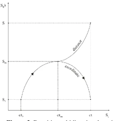
At rest: v (St) = v0 (St0) = 0. The graph of the function S = S (ct) is a straight line parallel to the axis ct (fig. 2). Then:
0
v 0 0 0
0
v
(
)
01
)
(
v
t tt t tt t s
S
dS
S
cdt
dS
dS
In this case the density of the space at the point of rest is infinitely large compared to the density of the time.
1. Movements on open trajectory.
a) Uniform motion (fig. 2).
We have: aτ (St) = aτ (t) = 0 V (St) = v0 (St0) = const
0
v v
In such case:
t t t t
t t
t t
t s
S
dS
S
dS
dS
dS
)
(
v
1
)
(
t t t t t t t t t t s
S
S
S
S
S
S
)
(
v
1
)
(
v
as the density of the space is the same along the entire trajectory:
s
s
const
, other than or equal to the density of the time.From two different uniform movements with speeds:
1 2
v
v
, in one and the same time interval, on thegreater speed corresponds less density of the space and vice versa:
1
v
v
2 1 1 2
s s
Figure 2: Densities at movements on open trajectory
b) Uniformly variable unidirectional motion (fig.2)
In this case: aτ(t) = const.
When: v0 > 0 , aτ > 0 - motion under constant acceleration;
v0 > 0 , aτ < 0 - motion under constant deceleration.
The laws on velocity and movement have the following type:
t
c
t
a
c
t
S
S
a
S
dS
S
a
S
S
t t t t t t t
)
(
)
(
v
)
(
)
(
v
)
(
)
(
v
)
(
v
0 0 0 0 0 0 2 0 0 0 0 2 0 0 0 0)
(
2
1
)
(
v
)
(
)
(
2
1
)
(
v
)
(
)
(
t
t
a
t
t
t
S
S
S
a
S
S
S
S
S
S
t t t t t t
Average velocity of the point is:
t
t
a
c
c
t
S
S
a
S
S
S
t tt t t
)
(
2
1
)
(
v
)
(
2
1
)
(
v
)
(
v
0 0 2 0 0 Respectively: t t t t t t t t t sS
dS
S
dS
dS
dS
)
(
v
1
)
(
v
t t t t t t t t t t sS
S
S
S
S
S
)
(
v
1
)
(
v
Here the density of the space is different at each point of the trajectory:
ρs = ρs(St)
as monotonously increases or decreases towards the density of the time.
c) Uniformly variable bidirectional motion (fig.3)
When the motion changes its direction on the trajectory
in point Sm (
v
m
0
tm
dS
dS
) - from uniformly
decelerating to uniformly accelerating in the opposite direction, the function S = S (St) is not monotonous. In this case we can proceed in two ways:
First Way:
According to [1] we divide the interval [ct0, ct] into two parts: [ct0, ctm] and [ctm, ct], where S(St) is a monotonous function and we consider the density of the space and time separately for each of them:
For the interval: [ct0, ctm]:
t t t t t s
S
S
d
S
d
)
(
v
1
t t t t t t sS
S
S
)
(
v
1
For the interval: [ctm, ct]:
t t t t t s
S
S
d
S
d
)
(
v
1
t t t t t t sS
S
S
as the differential densities of the space are not constant, and for the average densities we have:
1
v
v
s s
We have equality when: c[t0, tm] = c[tm, t].
Figure 3. Densities at bidirectional motion
Second way:
Instead of summary coordinate S, we can consider the law of covered distance S = S(St), which always is a monotonous function in the whole interval [ct0, ct]. Then in a similar manner define:
t t t t
t s
S
dS
dS
)
(
v
1
t t t t t
t s
S
S
S
)
(
v
1
2. Movements on a closed trajectory.
In general these are repetitive motions.
a) Uniform motion on a circle or ellipse (fig. 4a).
Let a material point moves uniformly in a circle with a radius R or in an ellipse with semi-axes a and b. Laws on velocity and covered distance respectively are:
const S
St)v(t) (
v 0 0
) )( ( v )
( v )
(SS0 SSS0 ttt0 Sttt
Respectively:
t t t t
t s
S
dS
dS
)
(
v
1
s
s
const
The movement is repeated with a period T, but the function S = S(St) is monotonous straight line across the whole interval t € [0, ∞] (fig. 4b).
Figure 4: Densities at movements on a closed trajectory When the movement is uneven: v = v (St) ≠ const. we have:
t t t t
t s
S
dS
dS
)
(
v
1
s(
S
t)
const
t t t t t
t s
S
S
S
)
(
v
1
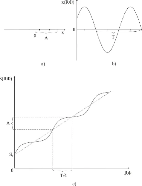
b) Harmonic oscillation of the material point.
Let a material point vibrate harmoniously along the axis Ox (fig. 5a). The laws of acceleration, velocity and motion are:
cos(
)
cos
)
(
t
2A
t
2A
a
x
sin(
)
sin
)
(
v
xt
A
t
A
cos(
)
cos
)
(
t
A
t
A
x
Where: ω – is a circular frequency of oscillation, A - amplitude, Φ = ωt + φ - phase of oscillation, φ - the initial phase.
In order to equalize the quality between the values of the function and argument we shall proceed as follows: [1]
The phase Φ has dimensionality of angle [rad]. In order to transform this dimension in length [m], we shall multiply it by the radius of the trigonometric circle R = 1 [m].
0 0SS
R S R R
S R R t
t R R t
R
R
dimensionalities of length [m]. Then the above laws acquire the type:
A
R
R
a
x(
)
2cos
A
R
R
)
sin
(
v
x
A
R
R
x
(
)
cos
The dimensionalities of vx and ах remain the same: [m/s] and [m/s2]. The graph of the function x = x (RΦ) is
shown in Figure 5. b. It is periodic with period:
T
2
.Figure 5: Densities at the harmonic oscillation Because of no monotony of function x = x(RΦ) we can divide the interval Δ(RΦ) on parts with a length equal to half-period, in which it is monotonous, or to consider the law on distance covered S = S(RΦ), which is monotonic function throughout the whole interval t € [0, ∞) and whose graph is shown in Fig. 5 c.
Then:
t t t
s
R
dS
R
dS
)
(
v
1
)
(
x
where the differential density of space varies periodically over time;
t t t t
s
R
S
R
S
)
(
v
1
)
(
x
where:
v
x(
R
)
2
A
is the average velocity in the interval of time: Δt = T/4.3. General case of an arbitrary motion.
Law on motion and law on velocity on the trajectory S have type:
t t t t t
t S SSaSdSdS S
S()0v0()
()
t t t
t S aSdS S)v() () (
v 0
Then:
t t t t t
t t t
t t
t t
t s
dS
S
a
S
S
dS
S
dS
dS
dS
(
)
)
(
v
1
)
(
v
1
)
(
v
0
t t t t t
t t
t t
t s
S
S
S
S
S
S
)
(
v
1
)
(
v
Or the density of the space is greater than, equal to or less than the density of the time. Change of ρs over time depends on the tangential acceleration of the point.
))
(
(
ts s
a
S
The condition of rest: v(St) = 0 has infinite density of the
space towards the density of the time.
III.
RESULTS AND DISCUSSION
1. On the ground of an arbitrary motion of a material point in classical kinematics the concepts density of time and density of space can be defined.
2. Because of the reversibility of the law of motion may be considered density of the space towards the density of time and vice versa - the density of time towards the density of space.
3. In all uniform motions the density of space is constant along the trajectory, greater than equal to or less than the density of the time. Its relative value is determined by the magnitude of the velocity of the point.
5. All uniform motions, in which the density of the space is constant, are reversible in time and space [4].
6. Classical motion of a material point allows only linear densities of space and time on the trajectory to be defined. In order to define the concepts of surface density and volume density of space and time the motion of multiple points must be considered simultaneously - continuously distributed in space environments.
7. Using the mathematical concept of the density of function [1] is a method that can be applied not only to the classical motion of a material point, but to all physical quantities, unique function of one or more variables.
8. In conclusion we shall receive an interesting function. We have above:
t t
t t
t s
t
c
S
dS
dS
)
(
v
)
(
v
1
Hence:
2 2
2 2
2 2
v
t st
dS
dS
c
In the four-dimensional space-time continuum in a special theory of relativity [5] four-dimensional interval is defined:
2 2 2 2
2 2 2 2 2 2 2 2 2
2
v
1
v
)
(
)
(
c
dt
c
dt
dt
c
dS
dt
c
cdt
idS
dl
where c is the velocity of light.
If we accept under the consideration prevailing hitherto for the normalizing velocity the velocity of light с, we can express the four-dimensional space through the density of space and time:
2 2 2 2 2 2 2
2
2 2 2
2 2 2 2 2 2 2
v
1
1
1
c
dt
c
dt
c
dS
dS
dS
dS
dS
dl
s t
s t t
s t t t t
Accepting of с = 3.108 m/s is resulting in that always: s
t
, as in the special theory of relativity: v < c.
IV.
REFERENCES
[1] A. Apostolov, Z. Peykov, Density of Function in the Mathematical Analysis, IJSRST, presented for publishing.
[2] Z. Peykov, A. Apostolov, Inversion of Space in the Classical Kinematics of Material Point, IJSRST, v. 2, No. 5, p. 309, 2016.
[3] Chr. Christov, Mathematical Methods in Physics, Nauka i izkustvo /Science and Art/, Sofia, 1967). [4] Z. Peykov, A. Apostolov, Inversion of Time and
Space in the Classical Kinematics of Material Point, IJSRST, v. 2, No. 5, p. 317, 2016.