Towards predictive data-driven simulations of wildfire spread – Part I: Reduced-cost Ensemble Kalman Filter based on a Polynomial Chaos surrogate model for parameter estimation

www.nat-hazards-earth-syst-sci.net/14/2951/2014/ doi:10.5194/nhess-14-2951-2014

© Author(s) 2014. CC Attribution 3.0 License.

Towards predictive data-driven simulations of wildfire

spread – Part I: Reduced-cost Ensemble Kalman Filter based

on a Polynomial Chaos surrogate model for parameter estimation

M. C. Rochoux1,2,3,4, S. Ricci1,2, D. Lucor5, B. Cuenot1, and A. Trouvé6 1_{CERFACS, 42 avenue Gaspard Coriolis, 31057 Toulouse Cedex 01, France}

2_{SUC/CNRS-URA1875, 42 avenue Gaspard Coriolis, 31057 Toulouse CEDEX 01, France} 3_{Ecole Centrale Paris, Grande voie des vignes, 92295 Châtenay-Malabry, France}

4_{EM2C/CNRS-UPR288, Grande voie des vignes, 92295 Châtenay-Malabry, France}

5_{Institut d’Alembert, Université Pierre et Marie Curie, CNRS-UMR7190, 4 place Jussieu, 75006 Paris, France} 6_{Dept. of Fire Protection Engineering, University of Maryland, College Park, MD 20742, USA}

Correspondence to: M. C. Rochoux ([email protected])

Received: 19 March 2014 – Published in Nat. Hazards Earth Syst. Sci. Discuss.: 9 May 2014 Revised: 2 September 2014 – Accepted: 23 September 2014 – Published: 10 November 2014

Abstract. This paper is the first part in a series of two articles and presents a data-driven wildfire simulator for forecasting wildfire spread scenarios, at a reduced computational cost that is consistent with operational systems. The prototype simulator features the following components: an Eulerian front propagation solver FIREFLY that adopts a regional-scale modeling viewpoint, treats wildfires as surface prop-agating fronts, and uses a description of the local rate of fire spread (ROS) as a function of environmental conditions based on Rothermel’s model; a series of airborne-like ob-servations of the fire front positions; and a data assimilation (DA) algorithm based on an ensemble Kalman filter (EnKF) for parameter estimation. This stochastic algorithm partly ac-counts for the nonlinearities between the input parameters of the semi-empirical ROS model and the fire front position, and is sequentially applied to provide a spatially uniform correction to wind and biomass fuel parameters as obser-vations become available. A wildfire spread simulator com-bined with an ensemble-based DA algorithm is therefore a promising approach to reduce uncertainties in the forecast position of the fire front and to introduce a paradigm-shift in the wildfire emergency response. In order to reduce the computational cost of the EnKF algorithm, a surrogate model based on a polynomial chaos (PC) expansion is used in place of the forward model FIREFLY in the resulting hybrid PC-EnKF algorithm. The performance of PC-EnKF and PC-PC-EnKF is

assessed on synthetically generated simple configurations of fire spread to provide valuable information and insight on the benefits of the PC-EnKF approach, as well as on a controlled grassland fire experiment. The results indicate that the pro-posed PC-EnKF algorithm features similar performance to the standard EnKF algorithm, but at a much reduced compu-tational cost. In particular, the re-analysis and forecast skills of DA strongly relate to the spatial and temporal variability of the errors in the ROS model parameters.

1 Introduction

takes full advantage of the recent technological advances for geo-referenced front-tracking becomes essential.

Despite our recent progress in computer-based wildfire spread modeling, our ability to accurately simulate the be-havior of wildfires remains limited because the underlying dynamics feature complex multi-physics processes occurring at multiple scales (Viegas, 2011). The dynamics of wildfires are determined by interactions between pyrolysis, combus-tion and flow dynamics, radiacombus-tion and conveccombus-tion heat trans-fer, as well as atmospheric dynamics and chemistry. These interactions occur at the following scales: vegetation scales that characterize the biomass fuel; topographical scales that characterize the terrain and vegetation boundary layer; and meteorological micro/meso-scales that characterize atmo-spheric conditions.

Relevant insight into wildfire dynamics has been obtained in recent years via detailed numerical simulations performed at flame scales (i.e., with a spatial resolution of the or-der of 1 m). For instance, FIRETEC (Linn et al., 2002) or WFDS (Mell et al., 2007) combine advanced physical mod-eling and classical methods of computational fluid dynam-ics (CFD) to accurately describe the combustion-related pro-cesses that control the fire behavior (e.g., thermal degradation of biomass fuel, buoyancy-induced flow, combustion, radia-tion and convecradia-tion heat transfer). Note that because of the high computational cost, flame-scale CFD is currently re-stricted to research projects (Linn et al., 2002; Mell et al., 2007; Rochoux, 2014) and is not compatible with opera-tional applications. In contrast, a regional-scale viewpoint (i.e., a viewpoint that considers scales ranging from a few tens of meters up to several kilometers) is adopted in the following: the fire is described as a two-dimensional front that self-propagates normal to itself into unburnt vegeta-tion; the local propagation speed is called the rate of spread (ROS). This viewpoint is the dominant approach used in current operational wildfire spread simulators, see for in-stance FARSITE (Finney, 1998), FOREFIRE (Filippi et al., 2009, 2013), PROMETHEUS (Tymstra et al., 2010) and PHOENIX RapidFire (Chong et al., 2013). In particular, FARSITE uses a model due to Rothermel (1972) that treats the ROS as a semi-empirical function of biomass fuel proper-ties associated with a pre-defined fuel category (i.e., the ver-tical thickness of the fuel layer, the fuel moisture content, the fuel particle surface-to-volume ratio, the fuel loading and the fuel particle mass density), topographical properties (i.e., the terrain slope) and meteorological properties (i.e., the wind velocity at mid-flame height). This approach is limited in scope because of the large uncertainties associated with the accuracy of computer models since they do not account for the interaction between the fire and the atmosphere, and since they have a limited domain of validity resulting from a cali-bration procedure based on experiments (Perry, 1998; Sulli-van, 2009; Viegas, 2011; Cruz and Alexander, 2013; Finney et al., 2013). This approach is also limited because of the large uncertainties associated with many of the input

param-eters to the fire problem (Jimenez et al., 2007; Finney et al., 2011).

of PC-based sampling techniques to problems of hyperbolic conservation laws remains a challenging task (Desprès et al., 2013).

Recent progress made in airborne remote sensing provides new ways to monitor real-time fire front positions (Wooster et al., 2005, 2013; Riggan and Robert, 2009; Paugam et al., 2013). Unfortunately, these thermal-infrared measurements provide an incomplete description of the fire spread (in par-ticular due to the opacity of the fire-induced thermal plume and/or due to a limited monitoring) and are subject to instru-mental errors as well as representativeness errors (i.e., incon-sistency between what the sensor can measure and what the computer model can describe). From this perspective, data assimilation (DA) offers a convenient framework for inte-grating fire sensor observations into a computer model in order to provide optimal estimates of poorly known model parameters and/or model state, and to improve in fine pre-dictions of the fire spread behavior (Mandel et al., 2008; Cowlard et al., 2010; Lautenberger, 2013; Rochoux, 2014). The key idea is that, when used alone, neither measurements nor computer models can provide a reliable and complete de-scription of the real state of the physical system. In the fol-lowing, the set of model state and/or model parameters to be corrected through DA is gathered in the control vector. The DA algorithm is sequentially applied; each sequence (also referred to as the assimilation cycle) is decomposed into two steps: (1) a prediction step, in which the control variables are advanced in time given some uncertainty ranges; and (2) an update step based on the classical Bayes’ theorem, in which new observations are considered and the probability density function (PDF) of the control variables is modified consis-tently with the observations in order to reduce the uncer-tainties in the model outputs (Gelb, 1974; Tarantola, 1987; Todling and Cohn, 1994; Ide et al., 1997; Kalnay, 2003; Re-ichle, 2008). The Kalman filter (KF) is the most commonly used sequential DA technique. However, the KF assumes lin-ear dynamics between the control variables and the model outputs as well as a Gaussian statistical distribution for both modeling and observation errors. Extensions of the KF that partly overcome these limitations have been proposed, for in-stance the extended Kalman filter (EKF) that uses local lin-earization techniques (Gelb, 1974) or the ensemble Kalman filter (EnKF) that relies on a stochastic description of the model behavior (Evensen, 1994, 2009). An insightful com-parison between EKF and EnKF is given within the frame-work of land DA in Reichle et al. (2002).

In this study, an ensemble-based DA methodology is con-sidered in order to reduce the uncertainties in the ROS model parameters using measurements of the time-evolving loca-tion of the fire front. This study is an extension of our previ-ous works presented in Rochoux et al. (2013a, b), in which a prototype data-driven wildfire simulator was developed. The initial prototype featured the following main components: an Eulerian front-tracking solver combined with a model de-scription of the local ROS proposed by Rothermel (1972);

a series of observations of the fire front position; and a cost-effective EKF-based DA algorithm. This prototype was suc-cessfully evaluated when applied for estimating the input pa-rameters of the Rothermel-based ROS model (e.g., the fuel moisture content, the fuel particle surface-to-volume ratio, and/or the wind direction and magnitude). However, the EKF algorithm relies on the assumption that the relation between a perturbation in the ROS model parameters and the result-ing changes in the fire front position (i.e., the generalized observation operator) can locally be approximated by a lin-ear relation. While the EKF-based studies presented in Ro-choux et al. (2013a, b) produced encouraging results and confirmed the value of a DA strategy for improved wild-fire spread predictions, the linearity assumption is no longer valid in regional-scale fires, especially when the wind direc-tion and magnitude vary and the vegetadirec-tion properties are po-tentially strongly heterogeneous. To better account for non-linearities in the generalized observation operator, an exten-sion to an EnKF approach was preliminarily explored in Ro-choux et al. (2012). This ensemble-based DA approach was originally developed for dynamic state estimation (Evensen, 1994) and has already been used in the field of wildfire mod-eling for correcting the temperature state variable (Beezley and Mandel, 2008; Mandel et al., 2008, 2011). It was also largely extended to sequential parameter estimation, for in-stance in the field of hydrology (Durand et al., 2008; Morad-khani et al., 2005). Still, the large number of realizations required by the EnKF algorithm to obtain satisfactory re-sults (Rochoux, 2014) may prove computationally burden-some within an operational framework. This behavior of the EnKF algorithm for parameter estimation is due to four main reasons: (1) the slow convergence rate of the Monte Carlo sampling; (2) the nonlinear interrelation between the con-trol space and the observation space; (3) the complexity of retrieving the specific signature of each control parameter on the resulting distribution of the simulated fire front; and (4) the accumulation of sampling errors along assimilation cycles that can only be addressed by increasing the size of the sample (Li and Xiu, 2008). The required size of the sam-ple significantly increases with the comsam-plexity of the physics (multi-parameter estimation) and the model nonlinearities (complex physics), thus emphasizing the need for a reduced-cost EnKF. Efforts have therefore been devoted to design-ing more efficient EnKF schemes by reducdesign-ing sampldesign-ing er-rors (Szunyogh et al., 2008; Saad, 2007; Li and Xiu, 2008, 2009; Blanchard et al., 2010; Xiu, 2010; Rosi´c et al., 2013). For this purpose, and following work from Li and Xiu (2009), an EnKF strategy based on a PC approximation (PC-EnKF) is proposed in this paper; the polynomial surrogate model be-ing used durbe-ing the EnKF prediction step to generate a large number of model simulation trajectories at almost no cost and without loss of accuracy (Birolleau et al., 2014).

of the Rothermel-based ROS model. The objective of this study is to show the feasibility of this approach for wildfire spread forecasting under several assumptions, i.e., a mini-malist treatment of the fire front (idealized as an interface and consistent with the limited knowledge on the environmen-tal conditions); a semi-empirical formulation of the ROS; Gaussianity of the errors on the input parameters of the ROS model and on the observations; prior values for the control parameters specified based on user-defined mean and error standard deviation (STD). In this first part, both the EnKF and PC-EnKF algorithms are limited to the estimation of spa-tially uniform parameters of the ROS model due to compu-tational cost constraints and a lack of high-resolution data on the environmental conditions. Although it seems appro-priate to translate the inability of a fire spread model to gen-erate accurate fire front positions into parameter uncertainty, other sources of uncertainties such as model structural er-rors or boundary/initial condition erer-rors also need to be ac-counted for. For this purpose, in the second part of this se-ries of two articles (Rochoux et al., 2014), a state estimation strategy is designed to address anisotropic uncertainties in wildfire spread as well as to provide observation-informed initial condition for model integration at future lead times. Thus, parameter estimation and state estimation are comple-mentary approaches that are valuable for wildfire behavior forecasting; it is therefore important to discuss their benefits and drawbacks for experiments with increasing complexity.

The outline of the paper is as follows. Section 2 presents the available observations of the fire behavior and the wild-fire spread model named FIREFLY (i.e., the forward model). The hybrid PC-EnKF algorithm developed for the wildfire application is presented in Sect. 3; in this section, the sequen-tial implementation of the ensemble-based algorithms is also described. Section 4 illustrates how the classical EnKF and the hybrid PC-EnKF allow to properly estimate model pa-rameters on simple test cases, in which the observations are synthetically generated. The performance of the data-driven wildfire spread capability using the reduced-cost approach is demonstrated in a validation test corresponding to a con-trolled grassland fire experiment.

2 Information on wildfires at regional scales: observations and forward model

2.1 Observations of the fire front location

2.1.1 Overview of available observations of fire spread In practice, continental surfaces and vegetation are mainly observed within the mid- and near-infrared regions of the electromagnetic spectrum of wavelengths (0.75 to 15 µm). It is known that for high temperatures as encountered in wild-fires (varying from 600 K for smoldering to 1200 K in the flaming zone), the maximum radiant intensity occurs within

the mid-infrared (MIR) region. Thus, current spaceborne and airborne systems observe wildfires within a narrow wave-band centered on the 3.9-micron wavelength (Butler et al., 2004; Wooster et al., 2005, 2013; Paugam et al., 2013; Ro-choux, 2014), which is both sensitive to flaming and smolder-ing combustion modes. Beyond fire detection, remote sens-ing is regarded as a promissens-ing approach to provide a quan-titative description of the fire radiation release to charac-terize sub-pixel fires (occupying a limited area of the sen-sor pixel down to 0.1 to 1 % of the pixel area) and to esti-mate fuel consumption as well as smoke emissions (Wooster et al., 2013). Using spaceborne or airborne platforms, the fire radiative power (FRP) emissions are detected in the burn-ing area, while non-active areas remain blank. This infor-mation is crucial to retrieve the brightness temperature and thus, to track the time-evolving location of the fire front. For instance, Paugam et al. (2013) showed that spatiotemporal variations of the flame front ROS can be accurately retrieved using FRP analysis on a reduced-scale controlled fire experi-ment (the final burnt area of the reduced-scale study is about 1000 m2); ongoing research aims at extending this FRP anal-ysis to regional-scale wildfire spread.1,2

Currently, most spaceborne instruments, including the pi-oneer generation such as the AVHRR (Advanced Very High Resolution Radiometer) and the MODIS (MOderate resolu-tion Imaging Spectroradiometer), offer neither a sufficiently short revisit period nor a high enough spatial resolution im-agery for efficient front-tracking at regional scales. While these objectives no longer seem out of reach for the dual SPOT-Pléiades constellation,3 airborne platforms still seem the most suitable solution for real-time geo-location of ac-tive fire contours. Typical examples are the LIVEFIRE sys-tem (Merlet, 2008; Crombette, 2010) and its US counterpart FIREMAPPER system deployed since 2004 by the US Forest Service and the US Department of Interior Bureau of Land Management (Riggan and Robert, 2009). As a complement, spaceborne data could be used for validation as well as cali-bration of models and DA procedures.

2.1.2 Choice of observations for data assimilation In the present study, we assume that observations of the fire front position are available and that these observations can be made at different relevant times with a low mea-surement error (typically, 0–30 m for the LIVEFIRE sys-tem). In the following, the observed fire front is represented as a segmented line using a pre-defined number of equally spaced markers (i.e., theN_froobservation markers); the obser-vation vector notedyo

t contains the two-dimensional

coordi-nates(x_io, y_io)of the fire front markers (the subscriptiis the 1_{http://wildfire.geog.kcl.ac.uk/}

2_{http://gofc-fire.umd.edu/}

c = 0

Front marker location (_xi, _yi)

c = 1

Γ

Burned region (c = 1)

Unburned region (c = 0)

Fire front (cfr= 0.5)

x

y

_Γ

n

α

α

w

u

w

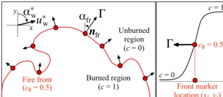
Figure 1. Eulerian front-tracking simulator FIREFLY. Left: the fire front is thecfr = 0.5 contour line;0measures the local ROS of the fire along the normal direction to the frontn_fr(defined by the direction angle of fire propagationαfr) given the wind velocity vec-tor (u∗_w, α∗_w). Right: profile of the spatial variations of the progress variablecacross the fire front, (xi, yi) representing the location of

theith fire front marker.

index of a particular marker in the observation vector, with

i=1,· · ·, N_fro) observed at the analysis timet. The size of the observation vectoryo_t is 2N_fro. The coordinates of the fire front markers are assumed to have independent Gaussian-like random errors o with zero mean and with STDσo. Note that this classical assumption of uncorrelated observation er-rors could be questionable. However, this aspect is out of the scope of this study and is still under active research in the DA field (Brankart et al., 2009; Gorin and Tsyrulnikov, 2011).

Two types of experiments are presented in the follow-ing: observation system simulation experiments (OSSE), in which observations are synthetically generated using a refer-ence solution of the FIREFLY fire spread model (called the true evolution) that is modified by random observation er-rorso; and a controlled grassland fire experiment, in which the observations are reconstructed from measured tempera-ture maps and using a definition of the fire front as the 600 K temperature contour line.

2.2 The fire spread model (the forward model)

The front-tracking solver, called FIREFLY and formally notedMin the following, simulates the propagation of sur-face wildfires within the biomass fuel bed and at regional scales, as illustrated in Fig. 1. Note that the present study is limited to flat terrains and problems with complex topogra-phy are outside its scope. FIREFLY tracks the time-evolving location of the fire front using the following three compo-nents: (1) a sub-model for the ROS noted0; (2) an Eulerian front-tracking solver for the fire front propagation equation; and (3) an isocontour algorithm for the reconstruction of the fire front.

2.2.1 The Rothermel-based rate of spread sub-model (a) Original one-dimensional formulation

The ROS sub-model is based on the widely used semi-empirical model due to Rothermel (1972) that describes0as a function of the local environmental conditions (e.g., veg-etation and weather properties). The ROS is derived from the one-dimensional formulation of the energy balance equa-tion per unit volume of the unburnt biomass fuel located ahead of the flame; the physical quantities involved in this energy balance are then parameterized using wind-tunnel ex-periments. In this formulation,0[m s−1] is expressed as the ratio between the heat flux received by the unburnt vegeta-tionIp[J m−2s−1] and the energy required to ignite the fuel

Hig[J m−3].0reads as follows:

0= Ip

Hig

= ξ Ir

ρbχ Qig

1+8w

. (1)

Ip is a function of the energy release rate of the combus-tionIr, of the dimensionless propagating flux ratioξ(that de-scribes the proportion of energy that is released by the flame and transferred to the vegetation in the non-flaming zone). The wind correction coefficient8w, which was determined for a one-dimensional case corresponding to a head fire con-figuration, nonlinearly depends on the wind velocity magni-tude at mid-flame heightuwsuch that

8w≡8w(uw)=CwuBww

_β

v

βv, opt

−Ew

, (2)

withCw, Bw and Ew calibrated parameters depending on the biomass fuel surface-to-volume ratio 6v [m−1], with

βv the biomass fuel packing ratio and βv, opt≡βv, opt(6v) its optimum value (optimum meaning thatβv,opt character-izes the optimum arrangement of the biomass fuel parti-cles that produces the most effective mixing between air and fuel gas reactants for the occurrence of combustion). The ignition energy Hig is formulated as Hig=ρbχ Qig, with

Qig [J kg−1] the heat of ignition, χ the dimensionless ef-fective heating number (i.e., amount of fuel efef-fectively in-volved in the ignition process) andρb[kg m−3] the biomass fuel bulk mass density that satisfiesρb=βvρpfor a porous medium,ρp[kg m−3] being the biomass fuel particle mass density.

The expression for the local ROS0due to Rothermel may be written in the following compact form that is equivalent to Eq. (1):

0≡0δv, Mv, Mv, ext, 6v, m00v, ρp, 1hc, uw

, (3)

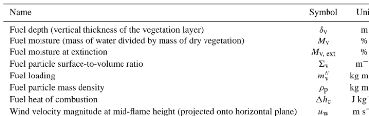
Table 1. Input parameters of the Rothermel-based ROS sub-model.

Name Symbol Unit

Fuel depth (vertical thickness of the vegetation layer) δv m Fuel moisture (mass of water divided by mass of dry vegetation) Mv %

Fuel moisture at extinction Mv, ext %

Fuel particle surface-to-volume ratio 6v m−1

Fuel loading m00_v kg m−2

Fuel particle mass density ρp kg m−3

Fuel heat of combustion 1hc J kg−1

Wind velocity magnitude at mid-flame height (projected onto horizontal plane) uw m s−1

(b) Extension to two-dimensional surface wildfire spread The original Rothermel’s one-dimensional model is extended to two-dimensional configurations, in order to account for the wind effects on the shape of the fireline, while still maintain-ing a simple parameterization of the ROS with respect to lo-cal environmental conditions. Accounting for wind-induced wildfire spread in FIREFLY is such that when the wind blows in the direction of the fire spread (i.e., a head fire configura-tion), the wind contribution to the ROS is maximum. On the contrary, the wind contribution to the ROS is zero when the wind blows in the direction opposite to the direction of the fire spread (i.e., a rear fire configuration), meaning that the fire propagates at the value of no-wind ROS on this section of the fire front (i.e., 8w=0). On the flanks, the fire front advances faster than in the absence of wind (i.e., 8w>0). This implies that the ROS can drastically change along the fireline at a given time. For this purpose, characteristic an-gles in the horizontal plane(x, y)are defined to represent the direction angle of the wind notedα∗_wand the direction angle of the fire propagation notedαfr(the index fr referring to the front);αfrindicates the outward-pointing normal direction to the fire front notednfr(see Fig. 1). These angles are defined from the northern direction, namely from the positivey co-ordinates and increasing in the clockwise direction. Since the propagation of wildfires is anisotropic, the normal vectornfr is not uniform along the fireline and is modified over time, with

nfr≡nfr(x, y, t )=

sinαfr(x, y, t ) cosαfr(x, y, t )

. (4)

Thus, the wind velocity magnitude at mid-flame heightuw (see Table 1) corresponds to the projection of the wind ve-locity vectoru∗

walong the normal direction to the frontnfr:

uw≡uw(x, y, t )=u∗w·nfr(x, y, t ), (5)

withu∗

wdefined by its magnitude,u∗w[m s−1], and direction angle,α∗_w[◦_]:

u∗_w=

u∗_wsinα_w∗ u∗_wcosα_w∗

. (6)

In the following,u∗_w andα_w∗ are treated as spatially uni-form and time-independent. The projected wind velocity at mid-flame height uw≡uw(x, y, t ) is a time-dependent and spatially varying quantity along the propagating fire-line. It is worth noting that the wind contribution 8w is forced to a zero-value in FIREFLY when the scalar prod-uctu∗_w · nfr(x, y, t )is negative (see Eq. 5) to ensure that the ROS0remains positive. This is consistent with the common assumption in the field of fire spread modeling that the fire propagates at least at the no-wind ROS. As for biomass fuel properties, the fuel depthδv≡δv(x, y) is treated as a time-independent, spatially varying quantity; all other ROS model parameters are treated as constant and uniform.

(c) Sensitivity study of the rate of spread

The identification of which parameters are important to in-clude in the control vector (denoted byx) is an essential step towards the application of DA to FIREFLY. The key idea when dealing with parameter estimation is to focus the cor-rection on a reduced set of parameters that have significant uncertainties and to which FIREFLY is the most sensitive.

In order to identify to which input parameters the ROS

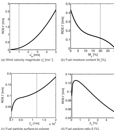
0is the most sensitive among biomass fuel properties and weather conditions, a sensitivity study is carried out with the classical one-dimensional Rothermel’s model for short grass. Nominal environmental conditions are as follows: the head fire propagates in presence of a moderate wind

u∗_w = 1 m s−1, and the vegetation is characterized by the moisture contentMv=20 %, the particle surface-to-volume ratio 6v=11 485 m−1, the layer thickness δv=0.5 m, and the layer packing ratio βv=0.106 %. These four parame-ters are perturbed around these nominal conditions. Note that the moisture at extinction Mv, ext=30 %, the fuel particle mass densityρp=512.6 kg m−3, the effective fuel mineral contentse=1 % (st=5.55 %), and the heat of combustion

1hc=1.861×107J kg−1remain constant and correspond to the standard values of the Rothermel’s fuel database (Rother-mel, 1972).

Figure 2 compares the variability in the ROS0when un-certainties are assumed in four parameters,u∗_w,Mv,6vand

u_w* _[m/s]

ROS

K

[m/s]

0 1 2 3 4 5

0 0.5 1 1.5 2 2.5 3

M_v [%]

ROS

K

[m/s]

0 5 10 15 20 25 30

0 0.1 0.2 0.3 0.4 0.5

Y_v [1/m]

ROS

K

[m/s]

0.1 0.5 1 1.5 2

x 104

0 0.05 0.1 0.15 0.2

`_v [%]

ROS

K

[m/s]

0 1 2 3 4 5

0.04 0.06 0.08 0.1 0.12 0.14 (a) Wind velocity magnitude u* _w [ms–1_].

(c) Fuel particle surface-to-volume

ratio ∑v [m–1].

(b) Fuel moisture content M_v [%].

(d) Fuel packing ratio β_v[%].

Figure 2. Sensitivity of the Rothermel-based ROS0to environmen-tal parameters; nominal conditions are indicated by vertical lines.

u∗_w. As for biomass fuel properties, they feature a wide scat-ter forMvand6v, while0is less sensitive toβv, indicating that a lack of information inu∗_w,Mvand6vresults in a sig-nificant uncertainty range in the ROS model predictions. It is also shown that the ROS 0 depends nonlinearly on the pair of parametersMvand6v; in particular, there is a ROS acceleration when the biomass fuel becomes drier or when the biomass fuel particles become thinner. Note that these nonlinearities are more important when the wind magnitude fluctuates over time or when the fire active area is covered by heterogeneous biomass fuels. This highlights the impor-tance of applying a DA methodology able to handle multiple sources of nonlinearities in the fire spread model.

2.2.2 The Eulerian front-tracking solver

An Eulerian front-tracking solver is used to propagate the fire front at the Rothermel-based ROS. FIREFLY adopts a classical approach taken from the premixed combustion lit-erature (Poinsot and Veynante, 2005), in which a reaction progress variable notedc≡c(x, y, t )is used as the prognos-tic variable of the solver and is introduced as a flame marker:

c=0 in the unburnt vegetation,c=1 in the burnt vegetation, and the flame front is identified as the contour linecfr=0.5 as illustrated in Fig. 1. In the Eulerian front propagation tech-nique, the progress variablecis calculated as a solution of the following propagation equation:

∂c

∂t = −γ · ∇c=0|∇c|, (7)

with0=γ ·nfrthe projected ROS given by Eq. (3) and de-fined along the normal direction to the fire front that satisfies nfr= −∇c/|∇c|.

Equation (7) is solved using a second-order Runge–Kutta scheme for time-integration and an advection algorithm for spatial discretization based on a second-order total varia-tion diminishing (TVD) scheme combined with a Superbee slope limiter (Rehm and McDermott, 2009; Mallet et al., 2009). Note that FIREFLY requires a two-dimensional field

c(x, y, t−1)as initial condition of any time period [t−1, t]. This initial condition is constructed such that the transition between c=0 and c=1 is smooth; a tangent hyperbolic function is used to represent this transition.

The validation of the FIREFLY Eulerian front-tracking solver was presented in prior works (Rochoux et al., 2013a; Rochoux, 2014). Model diagnostics were developed to en-sure the correct numerical behavior of FIREFLY. These di-agnostics were derived from the Kolmogorov–Petrovsky– Piskounov (KPP) analysis valid for uniform fuel condi-tions (Poinsot and Veynante, 2005) and extended to het-erogeneous biomass fuel for application to wildfire spread. They verify that the rate of change of the progress variablec

matches the average ROS along the fireline and also that the ROS at the head of the fire is consistent with the Rothermel’s 0-D formulation (see Eq. 3). In addition, they also verify that the front thickness, estimated as the average inverse of the maximum gradient ofc, remains small (i.e., a few mesh step-sizes) and relatively constant over time. In all tests performed to date, these diagnostics have showed the non-diffusive be-havior of the numerical scheme underlying FIREFLY, con-sistently with the physics of the fire spread problem. Further details are provided in Rochoux (2014).

2.2.3 Reconstruction of the simulated fire front and comparison with the observed fire front

Once the spatiotemporal variations of the progress reaction

care known, the position of the fire front is extracted using a simple isocontour algorithm such that, formally, the outputs of the FIREFLY model are as follows:

h

(xi, yi),1≤i≤Nfr

i

=M[t−1,t](ct−1, λ), (8)

where (xi, yi) represents the two-dimensional coordinates of the Nfr front markers obtained at timet (the index i indi-cating the marker), where ct−1 designates the initial con-dition (i.e., the spatial distribution of the progress variable

c at time (t−1)), and where λ designates the list of in-put parameters of the ROS model presented in Table 1,

λ=(δv, Mv, Mv, ext, 6v, m00v, ρp, 1hc, uw).

Simulated front

(c_fr = 0.5)

Observed front (x₁,y₁)

(x₂,y₂) (x₃,y₃)

(x₄,y₄)

(x₁O_,y 1

O₎

(x₂O_,y 2

O₎

d_t,1

d_t,2 c=0

c=1

Figure 3. Construction of the differences between simulated fire front (SFF) and observed fire front (OFF) noted dt= [dt,1,· · ·, dt,N_fro]. In this illustration,r=Nfr/N_fro=4.

(SFF) described by theNfrmarkers (corresponding to a fine-grained discretization of the front) and the observed fire front (OFF) at timet. Since observations of the fire front position are likely to be provided with a much coarser resolution and since they may cover only a fraction of the fire front perime-ter, the OFF is discretized with a set ofN_fromarkers such that the observation vectoryo_t reads:

yo_t =h(x₁o, y₁o), (x₂o, yo₂), . . . , (x_Noo fr, y

o

No fr)

i

, (9)

with N_fro much lower than Nfr. In order to compare SFF with OFF, a selection operator His introduced. This oper-ator pairs a subset of N_fro markers along SFF with theN_fro

markers along OFF, associating each marker of OFF with its closest neighbor along SFF (see Fig. 3). Preliminary tests re-ported in Rochoux (2014) have shown that a simple treat-ment (taking 1 out of everyrpoints) provides reasonable re-sults. Thus,N_fro=(Nfr/r), whereris an integer taking val-ues much larger than 1 that represents the difference in reso-lution between SFF and OFF. One of the advantages of this representation of the fire fronts is that it provides a local in-formation on the discrepancies between SFF and OFF, and not only a global information such as the difference in the burnt area or in the fireline perimeter. This local information is efficient at representing the anisotropy in wildfire spread.

It is worth noting that the topology of the fire front can be complex in real-world wildfire spread cases, and/or only a section of the fire front can be observed due to the opacity of the fire-induced thermal plume or due to a limited moni-toring. Thus, the pairing between simulated markers and ob-served markers becomes more challenging for complex fire front topology. The generalization of this treatment to com-plex fire front topology is out of the scope of this study.

It is also worth mentioning that the EnKF and PC-EnKF parameter estimation strategies presented in this paper are valid for any fire spread model; FIREFLY could readily be replaced by any other front-tracking wildfire spread simula-tor, for instance FARSITE, FOREFIRE, PROMETHEUS or PHOENIX RapidFire.

3 Data assimilation algorithm: the polynomial chaos-based ensemble Kalman filter

3.1 The standard ensemble Kalman filter

We present here the ensemble Kalman filter (EnKF) algo-rithm applied, in the context of parameter estimation, for one assimilation cycle between time (t−1) and timet.

3.1.1 Definition of the control space

The vectorxt ∈Rncorresponds to the control vector that

in-cludes thenuncertain parameters to be estimated over the assimilation cycle[t−1, t]. This implies that the location of the fire front is not estimated by the EnKF but is indirectly modified by integrating again the fire spread model over the time window [t−1, t] with the newly estimated control pa-rameters. Note that a parameter estimation approach can be considered by itself as an estimation problem and does not need to be combined with a state estimation approach to ob-tain an optimal EnKF (Pétron et al., 2002; Peters et al., 2005, 2007; Moradkhani et al., 2005; Durand et al., 2008; Ruiz et al., 2013a).

In the present study, the control parametersxtare assumed

global (i.e., spatially uniform) and constant over the time window [t−1, t]; they are only modified when moving to the next time window [t, t+1].

3.1.2 Generalized observation operator

The generalized observation operator Gt maps the control

space of xt onto the observation space of yot. Within the

framework of parameter estimation, Gt is a composition

of the fire spread modelM[t−1,t] (providing the Nfr front marker locations associated with a realization of the control vectorxt) with the selection operatorHt(taking 1 out of

ev-eryr=Nfr/N_fro markers along SFF at timet). Formally,Gt

reads:

yt=Gt(xt)=Ht◦M[t−1,t](ct−1, λ0,xt), (10)

withyt the location of theNfrofire front markers associated with a set of control parametersxtat timet(corresponding to

the model counterparts of the observed quantities), and with

λ0 the input parameters of the Rothermel-based model that are not included in the control vectorxt. In the following,

bothxt andyot are considered as random variables.

The observation operatorGt defined in Eq. (10) is

time-dependent since OFF is dynamically evolving: the selection procedureHt depends on the location and on the topology of

Cxy=Pt f

Gt T

xt

a,(k)

=xt

f,(k)

+Cxy(Cyy+R)

−1

(yt

o

+ξo,(k) −yt

f,(k)

) Prior parameters Prior fire fronts Posterior parameters

x

x

x

y

y

y

f,(Ne)

Covariance matrices

EnKF update

Cyy=GtPt

f

Gt

T

x

a,(1)

x

x

o

+ξo,(1)

Ke t Posterior fire fronts

y

y

y

prediction

FORECAST ANALYSIS

EnKF prediction

yt o

+ξo,(Ne) yt

o

+ξo,(2)

G

G

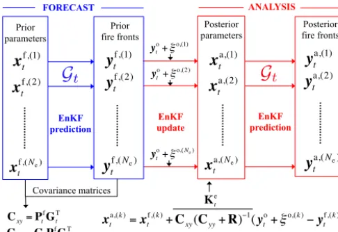
Figure 4. Flowchart of the EnKF algorithm during the [t−1, t] as-similation cycle for a parameter estimation approach. Data random-ization (Burgers et al., 1998) is used in the EnKF withξo,(k) fol-lowing observation error statistics for each memberk=1,· · ·, Ne.

3.1.3 Sequential estimation

The EnKF algorithm is sequentially applied over an assimi-lation window[t−1, t]; each assimilation cycle decomposes into two successive steps for each member of the ensemble indexed by the exponentkas illustrated in Fig. 4:

1. a prediction step (forecast), in which the system is evolved from time (t−1) to time t (t being the next observation time) through an integration of FIREFLY to forecast the fire front positionyt given some

uncer-tainty ranges in the control vector xt. We note pf(xt)

this PDF of the control vector (also called the forecast PDF) at timet. We also noteF[t−1,t] the operator

de-scribing the temporal evolution of the control parame-ters from time (t−1) to timet, withxt=F[t−1,t](xt−1). A temporal evolution of the control vector is introduced here to fit with the classical description of the EnKF al-gorithm: since there is no dynamic model available to describe the evolution of the control parameters, persis-tence forecasting is used to relate the forecast control parameters to the analysis control parameters (Peters et al., 2005). For this purpose, two techniques are re-ported in the literature, inflation on the one hand, a ran-dom walk model on the other hand (West, 1993; Morad-khani et al., 2005; Ruiz et al, 2013b). In this study, the parameter evolution modelF[t−1,t]is artificially set up

using a random walk model (see Eq. 23).

2. an update step (analysis), in which new observations are considered at the analysis timet and the forecast PDF of the control parameters is modified consistently with the observationsyo_t, in order to reduce the uncertainties in the computer model outputsyt. The new PDF, called

the analysis and noted pa(xt), is given by the classical

Bayes’ theorem:

pa(xt)∝p(yto|xt)pf(xt), (11)

where the symbol∝ means proportional to and where p(yo_t|xt)represents the data likelihood, i.e., the

condi-tional PDF of having the observationsyo_t given the con-trol vectorxt.

Based on Bayesian theory, the EnKF algorithm assumes that the errors on the control parametersxtand the errors on

the observationsyo_t are random variables defined by Gaus-sian PDFs with a zero mean value and an error covariance model. Under these assumptions, the forecast PDF may be written as follows:

pf(xt)∝exp

−1

2

xt−xft T

(Pf_t)−1xt−xft

, (12)

wherexf_t is the forecast estimate of the control vector, and where Pf_t∈_Rn×nis the forecast error covariance matrix rep-resenting errors in the ROS model parameters. The data like-lihood may be similarly expressed as follows:

p(yo_t|xt)∝exp

−1

2d T

t R

−1_d

t

, (13)

with R∈_R2Nfro×2Nfro the observation error covariance matrix representing observation errors (assumed constant over time in this study), and withdt the innovation vector of size 2N_fro

corresponding to the differences between SFF and OFF: dt=yot −y

f

t=y

o

t −Gt(xft). (14)

Using the selection procedure (see Fig. 3),d_t is simply de-fined as the vector formed by the directed distances between the paired SFF-OFF markers. Note that the statistical mo-ments ofdt(e.g., mean and STD) provide a convenient

mea-sure of the deviations of model predictions from observa-tions.

Within this framework, the analysis PDF from Eq. (11) is also Gaussian and is written as follows:

pa(xt)∝exp

−1

2

xt−xft T

(Pf_t)−1

xt−xft

−1

2d T

t R

−1_d

t , (15) ∝exp −1 2

xt−xat T

(Pa_t)−1xt−xat

, (16)

wherexa_t is the analysis estimate of the control vector, and where Pa_t ∈_Rn×n is the analysis error covariance matrix. Conditional mode estimation searches for the mode of the PDF pa(xt), i.e., the value of the control vectorxt that

equivalent to a minimization problem: max

xt∈Rn

pa(x_t)⇐⇒ min

xt∈Rn

−ln[pa(x_t)] = min

xt∈Rn

J(x_t), (17) withJ the cost function of the estimation problem defined as follows:

J(x_t)=1

2

x_t−xf_tT(Pf_t)−1x_t−xf_t+1

2d T

t (R)

−1_d

t. (18)

The direct minimization ofJ leads to the classical KF equa-tions when the generalized observation operatorGt is linear

(denoted by Gt). In the present case, this implies that the fire

spread modelM[t−1,t]is linear and that the parameter

evo-lution model F[t−1,t] is linear (denoted by F[t−1,t]). Using

these assumptions, it could be shown that the forecast in the prediction step is obtained via the integration of the follow-ing equations:

xf_t =F[t−1,t]xa_t−1, P f

t=F[t−1,t]Pf_t−1F T

[t−1,t], (19)

assuming there is no error in the formulation of the param-eter evolution model. In this context, the analysis update in Eq. (16) leads to the following equations:

xa_t =xf_t+Kt

yo_t −Gtxft

, (20)

Kt=PftGTt

GtPftGTt +R −1

, (21)

Pa_t =In−KtGt

Pf_t, (22)

where Ktis called the gain matrix. Starting from a prior value

of the control parameters (i.e., the forecastxf_t) and using the observationsyo_t available at timet, the analysis estimatexa_t is a feedback information for the fire spread model; xa_t is optimal when the variance of its distance to the true value xt_t gets to a minimum, meaning, for Gaussian cases, that its PDF is dense around its mean. The expressions in Eqs. (20– 22) are the basis of the EKF algorithm used in Rochoux et al. (2013a, b), F[t−1,t] and Gt being the tangent linear

opera-tors (Jacobian) ofF[t−1,t]andM[t−1,t]in the vicinity of the

control vectorxt, respectively. Thus, in the EKF, a linearized

and approximate equation is used for the prediction of errors statistics as well as for the relation between the control space and the observation space.

In contrast, the EnKF algorithm used in this study does not require the explicit use of the linear operators F[t−1,t]and Gt

in the prediction step. As shown in Fig. 4, the forecast control parametersxf_t are stochastically represented at timet based onNerealizations called the ensemble members

h

x_tf,(1),· · ·,x_tf,(k),· · ·,xf,(Ne) t

i ,

withkvarying between 1 andNe. These realizations are ran-domly generated based on mean and error STD according to the user-defined confidence interval for each control param-eter over the first assimilation cycle and to previous analysis

results for next assimilation cycles. The temporal evolution of the control parameters is artificially set up using a random walk model so that thek-th ensemble member reads: xf_t,(k)=F[t−1,t]

xa_t−,(k)₁=x_ta₋₁+e(k)_t−1, (23) wherexa_t−1is the mean of the posterior estimates obtained at the previous analysis time (t−1), and wheree(k)_t−1 is a ran-domly generated white noise following a Gaussian distribu-tion of zero mean and given STD (taken equal to the forecast error STDσf in the following). Thus, the generation of the ensemble of forecast parameters at timetis performed in two steps as in Peters et al. (2005): (1) the mean forecast estimate over the time window[t, t+1]is specified using the mean of the analysis estimates obtained over the previous assimilation cycle[t−1, t]; and (2) the ensemble of forecast parameters is obtained by applying a STD to this mean forecast estimate. Additionally, the error STD used in the random walk model remains constant over all assimilation cycles (Peters et al., 2005; Ruiz et al, 2013b). A series ofNeindependent forward model integrations up to the analysis timet based on these

Nerealizations of the control parameters is performed (start-ing from the same initial condition at time(t−1)that cor-responds to the mean of the posterior estimatesxa

t−1); this forecast step providesNe fire front positions at time t cor-responding to the model counterparts of the observed quan-tities and designated as[yf_t,(1),· · ·,yf_t,(k),· · ·,yf,(Ne)

t ], with

yf_t,(k)=Gt(xft,(k))for thekth ensemble member.

We note Cxy∈Rn×2N o

fr _{the matrix that represents the} stochastically based relation between the control space (of sizen) and the observation space (of size 2N_fro); Cxyis

ex-pressed as follows:

Cxy=PftGTt (24)

=

Ne X

k=1

x_tf,(k)−xf_t Gt(xtf,(k))−Gt(xft) T

Ne−1

,

where the overline denotes the mean value over the en-semble. Similarly, the symmetric error covariance matrix on the predicted measurements denoted by Cyy∈R2N

o fr×2Nfro _is stochastically formulated as follows:

Cyy=GtPftGTt (25)

=

Ne X

k=1

Gt(xft,(k))−Gt(xft) Gt(xft,(k))−Gt(xft) T

Ne−1

.

This means that the EnKF algorithm approximates the mean and the covariance of the forecast by the mean and the covari-ance of an ensemble, while still making the assumption that all PDFs are Gaussian. Additionally, the distance between the

kth predictionyf_t,(k)=Gt(xft,(k))and the observation vector

that an additional noiseξo,(k)is added to the observation vec-tor to avoid ensemble collapse. Thus, for thekth member, the innovation vectord(k)_t reads:

d(k)_t =yo_t +ξo,(k)−yf_t,(k). (26) During the analysis, each ensemble member is updated based on the classical KF formulation presented in Eqs. (20)–(22), with the difference than the generalized observation operator

Gt is nonlinear and that the gain matrix Ket is now

stochasti-cally calculated using Eqs. (24)–(25). Thekth member anal-ysis satisfies:

xa_t,(k)=xf_t,(k)+K_teyo_t +ξo,(k)−Gt

xf_t,(k), (27)

Ke_t =Cxy(Cyy+R)−1. (28)

One of the advantages of the EnKF formulation in Eqs. (27)– (28) is that the explicit estimation of the tangent-linear of the observation operator Gt (including the tangent-linear of the

fire spread model for parameter estimation) is avoided. This ensemble-based method allows the nonlinearity in the obser-vation operatorGtto be better taken into account than a local

estimation Gt achieved for instance through a finite

differ-ence scheme as in the EKF (Ros and Borga, 1997; Rochoux et al., 2013a, b). The use of Eqs. (27)–(28) provides an en-semble of posterior estimates at timet,

h

x_ta,(1),· · ·,x_ta,(k),· · ·,xa,(Ne) t

i ,

which is easily used to simulate over the time window[t−

1, t]an ensemble of retrospective posterior estimates of the fire front positions[ya_t,(1),· · ·,ya_t,(k),· · ·,ya,(Ne)

t ]as well as

an ensemble of forecasts of the fire spread beyond timet. Note that in the present study, we assume that observation errors are uncorrelated, i.e., the observation error covariance matrix R is treated as a diagonal matrix, in which each diag-onal term is the error variance(σo)2associated with the error in thex- ory-coordinate of the markers along OFF.

As a summary, the main steps of the proposed EnKF al-gorithm for parameter estimation over the assimilation cycle [t−1, t], are as follows:

1. build an ensemble of forecast control parameters based on Eq. (23), starting from the progress variable field cor-responding to the mean analysis field obtained at time (t−1);

2. compute the observation operator through Eq. (10), which includes the FIREFLY fire spread model integra-tion from time (t−1) to timet, in order to obtain the model counterparts of the observations at timet; 3. apply the Kalman filter update equation at timet for

each member of the ensemble based on Eqs. (24)–(28);

EnKF prediction

Surrogate model Surrogate model Forward model

Hermite quadrature Simulated fire fronts

Hermite polynomials Surrogate model

Forecast !

distribution! ➀!

Monte-Carlo sampling Predicted fire front positions

Posterior estimate of parameters

Updated fire front positions

➁

➂

EnKF update

('q)q= 1,· · ·, Npc

k= 1,· · ·, Ne

k= 1,· · ·, Ne

EnKF prediction k= 1,· · ·, Ne

k= 1,· · ·, Ne

FIREFLY

j= 1,· · ·,(Nquad)n j= 1,· · ·,(Nquad)n ⇣

xft,(j), !j

⌘ ⇣

yft,(j)

⌘

pf(xt)

yft=Gpc,t(xft)

⇣ xft,(k)

⌘

⇣ xat,(k)

⌘ ⇣

yat,(k)

⌘ ⇣

yft,(k)

⌘

Figure 5. Flowchart of the PC-EnKF algorithm during the assimila-tion cycle[t−1, t]decomposed into three steps: (1) construction of the PC expansion of the generalized observation operator; (2) EnKF prediction and update for the assimilation cycle[t−1, t]; and (3) pa-rameter evolution to the next assimilation cycle[t, t+1].

4. re-integrate the model Eq. (8) with the analysis parame-ters over the time period [t−1, t] to obtain the corrected locations of the fire front and the updated progress vari-able field at timet.

To move to the next assimilation cycle [t, t+1], step (1) can be performed again. The integration of the FIREFLY fire spread model starts again from the location of the fire front associated with the mean analysis estimate at timet, using the modified control parameters following the random walk model (see Eq. 23).

The proposed parameter estimation algorithm can be re-garded as a three-dimensional variational technique with a stochastically based estimation of the error covariance ma-trices; the three-dimensional variational technique also lacks the dynamic interrelation between analysis and forecast error covariances (Peters et al., 2005; Ruiz et al, 2013b).

3.2.1 General formulation of the surrogate model The PC-based surrogate model approximates the general-ized observation operator Gt at timet and is therefore

de-noted byGpc,t. It is parameterized with respect to the

multi-dimensional control vector xf_t∈_Rn following the forecast PDF pf(xt). This random vector may be regarded as a set of

second-order random variables (i.e., with finite variance) ex-pressed in terms of a random eventωsuch thatxf_t =xf_t(ω). It can be projected onto a stochastic space spanned by orthogo-nal PC functions of independent Gaussian random variables ζ(ω)as follows:

xf_t(ω)=

h

x₁f_,t, x₂f_,t,· · ·, x_nf_,t i

= ∞

X

q=0

ˆ

xqϕq

ζ(ω)

. (29)

The simulated positions of the fire frontyf

t=Gt(xft(ζ))can

also be viewed as a random variable and therefore, they can be projected onto a stochastic space spanned by orthogonal PC functions as follows:

yf_t =Gpc,t

xf_t(ζ)= ∞

X

q=0

ˆ

yq(t ) ϕq(ζ), (30)

where yˆq≡ ˆyq(t ) are time-dependent coefficients, and

where(ϕq)q=0,···,∞designate the multi-dimensional

approx-imating polynomial functions forming an orthogonal basis with respect to the joint PDF pf(xt)=pf(x1,t, x2,t,· · ·, xn,t).

The choice for the basis functions may depend on the type of random variable functions (Xiu and Karniadakis, 2002). Since the control vectorxf_t is assumed to follow a Gaussian PDF pf(x_t)within the framework of the EnKF, the surrogate model of the observation operatorGpc,t is built upon the

ba-sis of the Hermite polynomials (Ghanem and Spanos, 1991). Stated differently, the Hermite polynomials form the optimal basis for random variables following multi-variate Gaussian PDF. Note that the model outputsyf_t are represented in terms of the same random event ω as the model inputsxf_t, since the uncertainty in the model outputs is assumed to be mainly due to the uncertainty in the ROS model parameters within the framework of parameter estimation.

In practice, a truncated version of Eq. (30) is used; there are several ways of constructing the approximation space. The most common choice is to constrain the number of terms

Npcin the PC expansion by the number of control parame-ters nand by the maximum order of the polynomial basis

Qposuch that

Npc=

(n+Qpo)!

(n!Qpo!)

. (31)

This choice ofNpcensures that the PC approximation is of highest order Qpo. Note thatQpois a user-defined quantity that must be chosen carefully according to the model non-linearity, in order to obtain an accurate representation of the

model outputsyf_t with a high-order convergence rate. Theo-retically,Qpo=1 (i.e., only two terms forn=1 correspond-ing to the mean and STD of the control variable) is enough to approximate exactly a Gaussian random variable. Note also thatNpc rapidly grows withn andQpo, implying that a balance between accuracy and computational cost must be found. For instance, ifn=2 andQpo=2, there areNpc=6 terms retained in the PC expansion. Using this formalism, the surrogate modelGpc,tcan be formulated as follows:

yf_t∼=Gpc,t

xf_t(ζ)=

Npc X

q=0

ˆ

yq(t ) ϕq(ζ), (32)

where the unknowns are the following time-dependent vec-tors:

ˆ

yq ≡ ˆyq(t )= h

(xˆ1,yˆ1)q, . . . , (xˆNo fr,yˆNfro)q

i

t, (33)

qvarying between 1 andNpc, withNfrothe number of markers along OFF at timet. Note that the size of theqth vectoryˆqis

2N_fro(each marker location being represented with both the

x- andy-coordinate on the horizontal plane) and thereby, the computation of(2N_froNpc)coefficients (also referred to as the PC modes) is necessary to build the surrogate modelGpc,t.

3.2.2 Calculation of the polynomial chaos modes Due to the orthogonality of the PC basis, it can be shown that theqth PC coefficientsyˆqare given by the following:

ˆ

yq= E

h

Gpc,t(xft) ϕq(ζ) i

E h

ϕq(ζ)2i

, (34)

where

– E[·] refers to the expectation operator satisfying E[ϕq(ζ) ϕl(ζ)] =0 ifq6=l, with the following

defini-tion for the inner product:

E h

ϕq(ζ) ϕl(ζ) i

=

Z

Rn

ϕq(ζ) ϕl(ζ)p(ζ)dζ=δql

h ϕ_q2i,

(35) withδqlthe Kronecker delta-function;

– E[ϕq(ζ)2]is a normalization factor equal to 1 if the

ba-sis is constructed orthonormal;

– _E[Gpc,t(xtf) ϕq(xft)]is computed using a Gauss-Hermite

quadrature rule, with[xf_t,(1),· · ·,xf_t,(j ),· · ·,xf,((Nquad) n₎

t ]

such that 2Qpo≤2(Nquad−1). Thus, this term is com-puted as follows:

E h

Gpc,t(xft) ϕq(ζ) i

=

Z

Rn

Gt(xft) ϕq(ζ)dp(ζ) (36)

∼ =

(Nquad)n X

j=1

Gt(x

f,(j )

t ) ϕq(ζ(j )) w(j ),

where yf_t,(j )=G(xf_t,(j )) corresponds to the FIREFLY forward model integration evaluated at thejth quadra-ture root xf_t,(j ) with its associated weight w(j ), and where ϕq is the qth multi-dimensional basis function formulated as tensor products of one-dimensional poly-nomial functions:

ϕq≡ϕq(ζ)= n Y

l=1

ϕ1_i(l)Dζl

, (37)

withϕ_i(l)1Dthe one-dimensional polynomial basis and its multi-index i(l)varying between 0 and Qpo to deter-mine the proper term in the multi-variable space. Based on this formulation, the construction of the surro-gate modelGpc,t over the assimilation window[t−1, t]

re-quires a limited number of(Nquad)nforward model integra-tions (see the first step in Fig. 5). The polynomial approxima-tionGpc,tcalculated in Eq. (32) is then used in the prediction

step of the EnKF algorithm (instead of the observation op-erator Gt) to compute the predictions of the time-evolving

fire front locationsyf

pc,t for a large number of membersNe (see the second step in Fig. 5). This ensemble of forecasts is used to accurately estimate the covariance matrices Cxy

and Cyythat are required in the formulation of the Kalman

gain matrix. Thus, the EnKF update can be performed with reliable covariance matrices at a reduced computational cost compared to the standard EnKF algorithm based on a Monte Carlo sampling. This approach leads to analysis estimates of the control parametersxa_t,(k)and to accurate PDF of the fire front locations ya_t,(k) (k=1,· · ·, Ne) using the same surro-gate model as for the forecast estimates.

In order to reduce the computational cost of the EnKF al-gorithm, a surrogate model based on a PC expansion is used in place of the forward model (i.e., the FIREFLY regional-scale wildfire spread model) in the DA procedure. The per-formance of the resulting PC-EnKF algorithm is assessed on synthetically generated fire spread cases based on prelimi-nary work presented in Rochoux et al. (2012) as well as on the controlled grassland fire experiment.

3.3 Numerical implementation

In practice, the EnKF and PC-EnKF ensemble-based DA algorithms were implemented with the fire spread simula-tor FIREFLY using the OpenPALM dynamic coupling soft-ware (Lagarde et al., 2001), co-developed at CERFACS and

ONERA.4OpenPALM allows for the coupling of indepen-dent code components with a high-level of modularity in the data exchanges and treatment, while providing a straightfor-ward parallelization environment (Fouilloux and Piacentini, 1999; Buis et al., 2006). In this study, it is used as a task-parallelism manager to handle communications and data ex-changes between FIREFLY and the mathematical units re-quired to sequentially apply the EnKF and PC-EnKF algo-rithms. The PALM-PARASOL functionality in OpenPALM was used to efficiently and independently run the FIREFLY time-integrations in parallel, on the available processors. The master processor of PALM-PARASOL spawns multiple copies of the same computer program (i.e., the slaves), each on one or several processors with a different set of input pa-rameters of the ROS model. Each slave integrates FIREFLY using one realization of the control vectorxt to provide the

associated fire front positionyt, subsequently used for the

computation of the covariance matrices Cxyand Cyy. As

il-lustrated in Figs. 4 and 5, this integration is performed for theNe ensemble members using the forward model FIRE-FLY for the classical EnKF. In contrast, for the PC-EnKF al-gorithm, a limited number of FIREFLY model integrations

(Nquad)n is used to build the surrogate model and subse-quently, a large number of evaluations of the surrogate model (Ne) are computed using the PALM-PARASOL functional-ity.

4 Data assimilation experiments

4.1 Convergence of the ensemble-based algorithms The EnKF and PC-EnKF algorithms are compared on an OSSE experiment, in which the Rothermel-based ROS model of Eq. (3) is reformulated as0(x, y)=P δv(x, y)with

P [s−1_{]a proportionality coefficient andδ}

v≡δv(x, y)a spa-tially varying function that is assumed to be perfectly known. Note that this formulation takes advantage of the proportion-ality between the ROS0and the fuel layer thicknessδvin the Rothermel’s formulation. Thus, the control vector is limited to a single parameter,x=P, which encompasses different uncertainties that are not distinguished here.

The fire is ignited at(xign, yign)=(100 m,100 m)as a cir-cular front with a radius of 5 m; it spreads upon a random fuel distributionδv(x, y)over a 200 m×200 m domain. Observa-tions (represented usingN_fro=20 front markers) are synthet-ically generated at 50 s intervals with FIREFLY and a chosen true valuext_=Pt_{=0.4 s}−1_{. An observation error} character-ized by the error STDσois also introduced. The ensemble of prior values is drawn from a Gaussian distribution centered in xf=0.2 s−1_{with an error STDσ}f_{=0.05 s}−1_(assumed con-stant along the assimilation cycles). Note that the true value of the control parameter xtis at the tail of the Gaussian PDF associated with the forecast estimates. This case is chosen on

0 20 40 60 80 100 0.365

0.37 0.375 0.38 0.385 0.39 0.395 0.4 0.405

Number of members N e [−]

Mean of the analysis estimates [1/s]

Q_po = 4

Q_po = 2

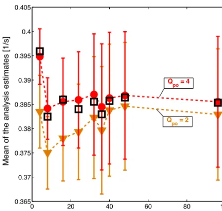
Figure 6. Convergence of the mean analysis estimates of the pro-portionality coefficientP [s−1]with respect to the number of en-semble membersNefor a fixed observation error STDσo=2 m and a single assimilation cycle: comparison of the performance between the EnKF and PC-EnKF algorithms. The orange triangled-dashed line corresponds toQpo=2; and the red circled-dashed line corre-sponds toQpo=4 for the PC-EnKF algorithm. Black squares cor-respond to the analysis estimates obtained using the standard EnKF. Vertical error bars correspond to the associated error STD.

purpose, in order to evaluate the ability of the parameter esti-mation approaches (EnKF and PC-EnKF) to retrieve accurate values of the control parameter, even though the prior value is far from the true control parameter and its uncertainty is high (compared to the observation error STD).

A PC approximation (with a polynomial order Qpo=4 and subsequently a quadrature orderNquad=5, see Sect. 3.2) is used to build the model response surfaceGpcto the control parameterx=P corresponding to the forecast(xf_{, σ}f_). 4.1.1 Sensitivity to sampling errors

Convergence properties of the EnKF-based analysis esti-mates are studied in Fig. 6 with respect to the number of ensemble members Ne for a fixed observation error STD

σo=2 m and for one assimilation cycle. Since there is no analytical solution to the problem, the convergence of the EnKF is assumed to be achieved if the mean value of the con-trol parameter and its STD remain constant when increasing

Ne. The performance of the PC-EnKF algorithm is compared to that of the standard EnKF algorithm (black squares) for different PC polynomial orders,Qpo=2 (orange triangled-dashed line) andQpo=4 (red circled-dashed line).

Figure 6 shows that in the present configuration, the EnKF algorithm converges for a minimum of Ne=48 members (meaning that FIREFLY is integrated 48 times to produce

48 fire front trajectories associated with each realization of the control parameter). In particular, below this threshold, the error bars corresponding to the error STD of the analy-sis parameter estimates are narrower for both EnKF and PC-EnKF algorithms. The error STD computed with a low num-ber of memnum-bers is therefore not reliable and the ensemble-based algorithms require a larger sample to accurately repre-sent the tails of the Gaussian PDF related to the control pa-rameterP. It is shown that the PC-EnKF algorithm provides a comparable result as the EnKF (in terms of mean and STD) above Ne=40 members for a polynomial order Qpo=4. However, the results achieved with PC-EnKF are obtained for a lower number of FIREFLY time-integrations (i.e., 5 FIREFLY model integrations only sinceNquad=5 quadra-ture points are used to build the model surface responseGpc) than the standard EnKF, while considering the same number of membersNe to generate the forecast/analysis estimates. Thus, the PC-EnKF algorithm provides a solution that re-produces the converged solution of the EnKF for a compu-tational cost that is reduced by a factor of at least 8. This implies that for more complex fire spread cases where more members are required to track spatial variations in wind and vegetation conditions, the PC-EnKF algorithm appears as a promising alternative to obtain accurate simulations of fire spread at a reasonable computational cost. Additionally, the PC-EnKF algorithm provides a mean estimate that is less fluctuating than the EnKF algorithm, with a slightly reduced scatter for low values of Ne, indicating that the PC-EnKF strategy requires less ensemble membersNeto reach conver-gence.

Figure 6 also illustrates the sensitivity of the PC-EnKF-based analysis to the choice of the PC polynomial order

Qpo for a varying number of ensemble membersNe. While

Qpo=2 (i.e.,Nquad=3) provides a reasonable approxima-tion of the mean analysis estimate when considering the standard EnKF as reference,Qpo=4 (i.e.,Nquad=5) leads to a more accurate estimate without loss of accuracy. Even though the fire front marker locations exhibit approximate Gaussian PDF and in theoryn=1 is sufficient to character-ize their distributions, a high polynomial order is required in this case. The true value (Pt=0.4 s−1) is indeed not in the zone of high probability occurrence of the forecast esti-mates (Pf=0.2 s−1withσf=0.05 s−1); the true fire front locations are at the tail of the forecast PDF, which makes the estimation of the fire front locations more difficult. This diffi-culty shows the ability of the PC-EnKF procedure to retrieve accurate estimates of the fire spread at a low computational cost and without loss of accuracy, even though the prior in-formation is very uncertain.

4.1.2 Example of polynomial chaos-based surface response