© European Geosciences Union 2002
and Earth
System Sciences
Simulation of the effect of defence structures on granular flows
using SPH
P. Lachamp, T. Faug, M. Naaim, and D. Laigle
Cemagref ETNA, Domaine universitaire BP 76, 38402 Saint-Martin d’H`eres Cedex, France Received: 20 September 2001 – Revised: 19 February 2002 – Accepted: 23 April 2002
Abstract. This paper presents the SPH (Smoothed Particles Hydrodynamics) numerical method adapted to complex rhe-ology and free surface flow. It has been developped to sim-ulate the local effect of a simple obstacle on a granular flow. We have introduced this specific rheology to the classical for-malism of the method and thanks to experimental devices, we were able to validate the results. Two viscosity values have been simultaneously computed to simulate “plugs” and “dead zone” with the same code. First, some experiments have been done on a simple inclined slope to show the accu-racy of the numerical results. We have fixed the mass flow rate to see the variations of the flow depth according to the channel slope. Then we put a weir to block the flow and we analysed the dependence between the obstacle height and the length of influence upstream from the obstacle. After hav-ing shown that numerical results were consistent, we have studied speed profiles and pressure impact on the structure. Also results with any topography will be presented. This will have a great interest to study real flow over natural topogra-phy while using the model for decision help.
1 Introduction
This article deals with the application of Smoothed Parti-cle Hydrodynamics (SPH) to the study of granular flows over rigid obstacles down an inclined channel. The inter-action between an obstacle and the flow is extremely im-portant to investigate the influence of singularities in terms of energy dissipation, bypassing... We will focus interest on the modification of the flow resulting from the presence of a weir and especially on the zone of influence upstream of the structure. The application of this study is dedicated mainly to the improvement of defence structures against dry snow avalanches and granular debris-flows. In that aim, we will consider a Mohr-Coulomb rheology, classically used
Correspondence to: P. Lachamp
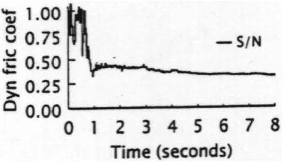
for granular debris-flows and which can tentatively be used for dry-snow avalanches considering as Naaim and Naaim-Bouvet (2000) and Dent et al. (1998) that natural flows ex-hibit a dependence between normal and tangential stresses in that case (Fig. 1).
The Mohr-Coulomb model assumes that the ratio tangen-tial to normal stress is a constant depending on the internal friction angle of the material. In our case, we will use glass beads whose value of internal friction angle is about 27◦. For this material, previous studies have shown Pouliquen (1999) that steady uniform flows exist only inside a small range of channel slope. We consider here a slope angle inside the range 29◦to 32◦(θ=30◦is chosen in practice). To carry out laboratory experiments, we must take into account similarity criteria and especially the Froude numberF r= √u
gh, where
uis the mean velocity, hthe flow depth andg the gravity. Snow avalanches generally have a Froude number ranging from 1 to 5 (Ancey, 1997), while granular debris-flows gen-erally have a Froude number close to 1. The mass flow rate must be adjusted to obtain values ofuandhcoherent with these criteria. We will present first the numerical method, the rheological model, the way it is considered in the model, the state equation and the boundary conditions that are used. In a second time, we will present the validation of the model and its use to show interesting data inside the flow that we can’t obtain experimentally. In a third time, the adaptation of the model to any type of topography will be presented.
2 Numerical method
2.1 General presentation
sim-Fig. 1. Results of experiments (Dent et al., 1998) with snow: NS = cst e.
ulate flows of incompressible fluids we will consider them as weakly compressible fluids. In that way, we are going to solve the momentum equation for incompressible fluids Eq. (2) but in the same time, the conservation of the mass will be solved thanks Eq. (3). This method is the most often used even when considering compressible flows (Monaghan, 1988; Gingold and Monaghan, 1983). The advantage of the SPH method is that it allows a three-dimensional approach without too much complexity and furthermore the position of the free surface for gravity-driven flows is easily com-puted. The model being three-dimensional, pressure and ve-locities (two essential variables in the framework of the study of flow-structure interactions) can be computed locally. Pres-sure is computed using a state equation which takes into ac-count both hydrostatic and dynamic effects.
2.2 SPH equations 2.2.1 Classical formalism
Equations of motion are determined on the basis of the clas-sical continuity equation for fluids interpolated on a mesh structure based on the position of the particles. The mesh, initially organised, rapidly becomes disorganised. The inter-polation is based upon a classical quadrature technique using a cut-off function whose limit is a Dirac around the consid-ered particle. The most common cut-off function Monaghan (1989) writes:
W (s)= C
hλ
1−3s2 2 +
3s3
4 ,0≤s≤1 1
4(2−s)
3,1≤s≤2 0, s ≥2.
(1)
wheres= krk
h (r = krkis the distance between two particles
andh depends on the initial spatial step 1x: for the 2-D case,h '1.21x),λis the dimension of space andC takes the values 23, 710π, π1, respectively forλ = 1,2 or 3. This polynomial form provides a strictly compact support to the cut-off functionW. Let us consider the classical equations of the fluid mechanics. We have:
du
dt =∇·
1
ρσ
+F (2)
∂ρ
∂t = ∇ ·(ρu) (3)
For free-surface flows, the source termF reduces to gravity, uis the velocity vector andσ is the full Cauchy tensor (in-cluding pressure and deviatoric parts). We will come back later to the definition of this tensor (see Sect. 2.2.2). When no viscosity of the fluid is considered, Eqs. (2) and (3) can be rewritten as:
duα
dt =
X
β∈G
mβ
σ (α)
ρ2
α
+σ (β)
ρβ2
−5αβI
∇αWαβ+g (4)
∂ρ ∂t =
X
β∈G
mβuαβ.∇αWαβ (5)
in which each particleα(resp.β) has a massmα (resp.mβ),
a velocityuα (resp. uβ), a stress tensorσ (α)(resp. σ (β))
and a densityρα (resp. ρβ). Gis the set of particle in the
domain of interest.I is the identity tensor. The derivative of
Walong coordinates of particleαwrites:
∂Wαβ ∂xi α = ∂ ∂xi α
Wrαβ h
(6) where rαβ = krαβkis the distance between particle αand
particleβ. The exponantidesignates any coordinates. And (Monaghan and Gingold, 1983)
5αβ =
−acµαβ+bµ2αβ
ραβ∗ ,uαβ.rαβ <0
0,uαβ.rαβ≥0
(7)
is a numerical viscous pressure possibly used when shocks, for instance, are considered. For the treatment of free-surface flows, we choosea=0.01,b =0 and, in Eq. (8),η=0.1h
(Monaghan, 1994). uαβ is the difference between the two
speed vectorsuαβ=uα−uβ.cis the “average speed sound”
of particlesα andβ. In our simulations, we considered a constant value of the parameterc(see Sects. 2.3 and 2.5). In Eq. (7),
µαβ=
huαβ.rαβ
rαβ2 +η2 (8)
ραβ∗ is the average value of the density between particlesα
andβ(i.e.ραβ∗ =mαρα+mβρβ
mα+mβ ).
2.2.2 Introduction of the fluid behaviour in SPH method The formalism of SPH considering the Mohr-Coulomb rhe-ology has been introduced by Savage, Oger and Gutfraind (Oger and Savage, 1999; Gutfraind and Savage, 1997) for the study of ice floes drifting under the action of the wind. The rheology is considered through the use of an apparent viscos-ity based on the assumption that principal axes of stress and strain rates are collinear. Thus, the apparent viscosityζα of
particleαwrites
ζα = min
(Pα+σa)sinφ
| ˙1(α)− ˙2(α)| , ζmax
˙
1(α)and˙2(α) are the principal components of the strain rate tensor of particle α (i.e. (α)˙ is defined later), σa is
a possible cohesion. φis in our case the internal frictional angle of the used material (some numerical data are given in Sect. 3.1). Furthermore, it should be noted that the pressure
Pα, the cohesionσaand the angleφtake only positive values.
Expression (9) leads to two different types of behaviour: whenζα < ζmax, particleαhas a plastic behaviour and when ζα =ζmax, it has a viscous behaviour.
This apparent viscosity is introduced through the follow-ing viscoplastic model Eq. (10):
σij(α)= −Pαδij+2ζα
˙
ij(α)−
1
2˙kk(α)δij
(10) ˙
(α)is the strain rate tensor of particleαthat we classicaly define by(α)˙ = 1
2
∇uα +(∇uα)t
. Thanks to Eq. (10), we can define the shear stress by Eq. (11):
τα =σ12(α)sinφ (11)
To increase the time step, we have chosen to distinguish two cases: one for which the strain rate and the velocity are equal to zero (dead zone) and one for which the strain rate is zero and the velocity is constant but not equal to zero (plug). To achieve that, we introduce a critical velocityvcso that
ζα = min
(Pα+σa)sinφ | ˙1(α)− ˙2(α)|, ζ
0 max
,kuαk< vc
ζα = min
(Pα+σa)sinφ | ˙1(α)− ˙2(α)|, ζ
1 max
,kuαk ≥vc
(12)
Thus,ζmax0 ζmax1 . To choose the values of these param-eters, we come back to the definition of the rheology (that allows us to determine the mean velocity inside the zone of interest). It was possible to find a consistent value forvc. To
determine the values ofζmax0 andζmax1 , we can approximate the average value of˙ inside the boundary layer to estimate its size (see Sect. 2.5). This technique is worthwhile to stop the particles inside the “dead zone”.
We can finally write the equation of motion considering normalσand shearτ stresses.
duiα dt =
X
β∈G
mβ
σii(α)
ρ2
α
+σii(β)
ρ2β −5αβ
∂Wαβ
∂xi α
+X
β∈G
mβ
τα
ρ2
α
+τβ
ρβ2
∂Wαβ
∂xαj
+gi (13)
iandj designate any components (i 6= j). In that way, for our 2-D cases, we have a set of two equations (one for each component of the speed vector).
2.3 The equation of state
As stated before, even incompressible fluids must be treated as weakly compressible fluids in the framework of SPH method. Thus, the pressure must be computed at each point. The pressure should be determined thanks the following Eq. (14).
Pα = −
1 2
σ11(α)+σ22(α)
(14)
But in our case, it’s impossible to solve simultaneously Eqs. (10) and (14). In this aim, we use a thermodynamic ap-proach. We introduce an equation of state which determines the pressure value on the basis of the density and writes (Monaghan, 1989):
Pα =P0+c2(ρα−ρ0) (15)
First, the relation∂Pα
∂ρα =c
2is verified. Furthermore, we con-sider that the compressibility and the speed sound are linked by1ρα
ρα =M 2
α (i.e.Mαis the Mach number of particleαand
is defined byMα = kucαk). In that way, the compressibility
of particleαis defined by1ρα = ρα.Mα2and if the sound
speed is around ten times the maximal value of the flow, the maximal compressibility will be around one per cent.
We can determine the dynamic pressure asPα =ραkuαk2
which is computed with the real instantaneous density and not an average one that should be constant. Let us remark that the pressure does not depend on the sound speedc, thus we are allowed to choose a low (non physical) value ofc
to increase the time step in the application of the numerical method. Numerical data will be developed in Sect. 2.5. 2.4 Boundary conditions
The boundary conditions are quite easy as long as simula-tions concern flows on a flat surface. But when accelerasimula-tions like the effect of gravity are considered, problems appear in the vicinity of boundaries. Lots of different techniques have been applied in previous works to take into account the effect of the boundary. Here, we consider the force that applies to a particle writes, forr≤r0(Monaghan, 1994):
f (r)=D
r0
r
p1 −r0
r
p2r
r2 (16)
and f(r) set to 0 ifr > r0.D =kgH, 1≤k ≤10,Hbeing the initial height of the fluid in the case of a dam break.ris the distance between the considered particle and the bound-ary,r0=1x.p1andp2are chosen to be respectivly 4 and 2 (Monaghan, 1994). But this expression is not fully compat-ible with the pressure inside the fluid. In fact the repulsive force and the pressure at the boundary have to be compati-ble. Thus, we must satisfy the following expression:
Z
f (z)φ (x, z)dxdz=
Z
∂
P φ (x,0)dx (17)
is the spatial domain and∂its boundary.φEq. (17) must be verified for any value ofx. In that way, we can simplify this condition:R
f (z)dz=P. This is the continuous form of the compatibility relation. Then the discret form of Eq. (17) writes:
X
f φ1x1z=XP φ1x (18)
If we now assume that only one layer of particles interacts with the boundary, each sum in Eq. (18) reduces to one term:
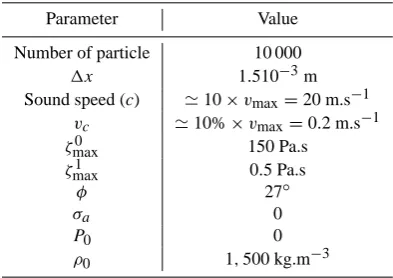
Table 1. Some numerical parameter values
Parameter Value Number of particle 10 000
1x 1.510−3m
Sound speed (c) '10×vmax=20 m.s−1 vc '10%×vmax=0.2 m.s−1 ζmax0 150 Pa.s
ζmax1 0.5 Pa.s
φ 27◦
σa 0
P0 0
ρ0 1,500 kg.m−3
so thatf = P
1z. In the two-dimensional case,1z=1x =
q
m
ρ and we can define the body force by a constant
depend-ing on the local pressure, density and mass by:
f = P
qm
ρ
(20)
All the calculation has been done without considering any particle. In fact, the applied force should be written:
fα=
Pα
q
mα
ρα
nα (21)
in whichfα is the force that must be applied to the particle
αandnαis a unit normal vector according to particleα. We
can note thatfα depends on the distance to the boundary
through the values of the mass, the density and the pressure. 2.5 Initial numerical conditions
Numerical parameters values used in the code are presented in the following table (Table 1).
3 Results
3.1 Comparison with experimental data 3.1.1 Presentation of the experimental device
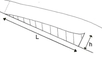
Experiments were carried in a laboratory inclined flume, two meters long and five centimeters wide (Fig. 2). Pumps circu-late material (sand or glass beads) with a mass flow rate rang-ing from 0.3 to 1.5 kg.s−1. For this kind of material, some steady uniform flow may occur only inside a narrow range of channel slope which depends essentially on the internal fric-tion angle. For glass beads, the internal fricfric-tion angle is 27◦ and the considered slope ranges from 29◦to 33◦.
Fig. 2. Experimental device.
3.1.2 The simplest configuration
First, we have tested the code without any obstacle for differ-ent channel slopes. In that way, we were able to quantify the depth of the flow depending on the channel slope by keep-ing a constant mass flow rate. This test has been made to control the chosen behaviour law. The mass flow rate was fixed atQm =0.35 kg.m−3(depending only on the size of
the hopper exit at the top of the channel). Results are shown on Fig. 3. In that case, we are not obliged to compute both viscosities. In fact, we have no “dead zone” except in the hopper but it doesn’t matter. It has permitted us to determine the value ofζmax1 . The maximal speedvmax(at the free sur-face) is around 2 m.s−1and the flow is between one and two centimeters deep (dis the depth of the flow). In the follow-ing equation,pdesignates the relative pressure exerted by a column of fluid. Thus we may estimate
ζmax1 = vp max
d
'ρgd 2
vmax = ρgd
3
Qm
'0.5 Pa.s (22)
3.1.3 Data of interest and validation
Fig. 3. Flow depth versus channel slope for a fixed mass flow rate.
Fig. 4. Measured lengths L andhobs
of the dead zone versus the heighthobsof the obstacle
result-ing from experiments and from simulations. In that case, we have to estimateζmax0 . By introducing the critical speedvc
(see Table 1), we can write:
ζmax0 'ρgdv c
d
'150 Pa.s (23)
It can be seen in Fig. 5 that experimental and computed points are very close to each other. Most of the points were obtained for low height of the obstacle because simulating a very long flume was too much time-consuming. However, this first result allows us to conclude that the model is con-sistent with the observations.
3.2 Pressure and velocity profiles 3.2.1 Results
The main interest of the method presented here is the accu-racy of the computation close to singularities. With classical numerical methods using grids of the spatial domain, it is necessary to refine the size of grids to control large evolu-tions of dynamic variables. With SPH we get some informa-tion on the pressure, density and velocity for each particle location. Thus, we are able to compute correctly the veloc-ity profile (Fig. 6) everywhere in the flume, and especially around obstacles. Figure 6 brings us information concerning
Fig. 5. Comparison between numerical and experimental results.
Fig. 6. Velocity profile above the obstacle.
the use of two different viscosities: in fact, in that case, the obstacle height ishobs =10−2m. Just before the obstacle,
particles are quite stopped: the average speed is around 0.05 m.s−1. Above this “dead zone”, we can observe a strong shear: speeds increase almost linearly. The last five centime-ters constitute a “plug”: the speed is constant over a certain height (around 6.10−3m). Otherwise, we can plot the pres-sure as a function of time: for specialists of structures, the evolution in time of the maximum pressure (Fig. 7) on the obstacle is a very interesting data. Figure 6 and Fig. 7 clearly demonstrate the capabilities of SPH numerical method to represent free surface flows of granular material. We can ob-serve that all data are quite regular with no exceptional sin-gularity. Velocity and pressure are the most interesting data but we could have also plotted density profiles.
3.2.2 Comparison with engineering laws
Fig. 7.Pmax(Pa) versus time around the obstacle.
kmust be chosen around 1 and 2. In fact, while designing defence structures, engineers are used to consider a value of
kbetween 1 and 4. In terms of value, results seem to be quite well. But the most important information is based on the duration of this sollicitation. And this is actually the main result of this numerical modelling. Up to now, we don’t have any other results to compare ours.
4 Flows over a complex topography
After the simulation of flows in basic geometry we will see now how to take into account complex topographies. The aim of this part is to establish how to simulate a flow over a topography represented by a DTM. There are two ways to define the topography. The first one is to build up a grid of the boundary using supplementary particles which will in-teract with the fluid particles. This method is interesting to represent the frictional effect but is quite time consuming. Another way consists in building up a grid of the spatial do-main. We present here the two-dimensional case. Let us define the topography between two abscissasxminandxmax and separate this domain into N-1 intervals. We assume the elevationzi =z(xi)is known for eachi(0≤i≤N). Then
we can compute the elevation along each line using the fol-lowing expression:
z= zi+1−zi
xi+1−xi
(x−xi)+zi (24)
Knowing the coordinates(xα, zα)of fluid particleα, we can
estimate the distance between this particle and the boundary and then determine if the body forcefα defined in Eq. (21)
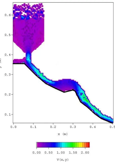
must be applied. Up to now, only two-dimensional flows (Fig. 8) have been considered but the same technique could easily be applied to three-dimensional flows. We did not carry out any validation of the result but at least we can anal-yse it qualitatively. In the hopper, the velocity is almost zero
Fig. 8. Velocity field over a complex topography.
everywhere. In zones where the slope reduces, the velocity diminishes and for steeper slopes, the flow shows a sheared zone close to the boundary and an unsheared zone (“plug”) close to the free surface. Qualitatively, all these results are consistent.
5 Discussion and conclusion
of the order of magnitude of collisional dissipations between particles. Even if the body force is determined according to the pressure, the acceleration imposed to particles when they are close to the boundary generates a normal speed that cannot be neglected. The consequence of this effect is phys-ically close to collisions that take place in the real flow, thus leading to flow height and velocities coherent with the mass flow rate and slope of the flume. Further use of the model requires some more validations with other mass flow rates and slopes of the flume. A sensitivity analysis should be carried out. In the near future, a similar work will be car-ried out with yield-stress fluids (Herschel-Bulkley) to simu-late muddy debris-flows. Thus the model will be able to treat both simple and complex rheological behaviours over any to-pography, leading to a complete tool dedicated to the study of snow avalanche structures and debris-flow structures in-teractions.
References
Ancey, C.: Rh´eologie des ´ecoulements granulaires en cisaillement simple, Application aux laves torrentielles granulaires, PhD the-sis, Ecole Centrale de Paris, 1997.
Dent, J. D., Shmidt, D. S., Louge, M. Y., Adams, E. E., and Jazbutis, T.G.: Density, velocity and friction measurements in a dry-snow avalanche, Annals of Glaciology, 26, 247–252, 1998.
Gingold, R. A. and Monaghan, J.J.: Shock simulation by the parti-cle method SPH, Mon. Not. Roy. Astr. Soc., 204, 715, 1983. Gutfraind, R. and Savage, S. B.: Smoothed Particle
Hydrodynam-ics for the simulation of broken-ice fields: Mohr-Coulomb type rheology and frictionel boundary conditions, J. of Comp. Phys., 134, 203–215, 1997.
Lucy, L. B.: A numerical approach to the testing of the fission hy-pothesis, Astron. J., 83, 1013, 1977.
Monaghan, J. J. and Gingold, R. A.: Shock simulation by the parti-cle method SPH, J. of Comp. Phys., 52, 374–389, 1983. Monaghan, J. J.: An introduction to SPH, Comp. Phys. Comm., 48,
89, 1988.
Monaghan, J.J.: On the problem of penetration in the particle meth-ods, J. of Comp. Phys., 82, 1, 1989.
Monaghan, J. J.: Simulating free surface flow using SPH, J. of Comp. Phys., 110, 399–406, 1994.
Naaim, M. and Naaim-Bouvet, F.: La neige: recherche et r´eglementation, 169, 2000.
Oger, L. and Savage, S. B.: Smoothed Particle Hydrodynamics for cohesive grains, Comp. Meth. in Applies Mech. and Eng., 180, 169–183, 1999.