IJPAS Vol.03 Issue-12, (December, 2016) ISSN: 2394-5710 International Journal in Physical & Applied Sciences (Impact Factor- 4.657)

(1)

Sample Size for Testing the Homogeneity of Several Normal Population Variances

M. Pran Kumar1 and G. V. S. R. Anjaneyulu2

Department of Statistics, Acharya Nagarjuna University GUNTUR – 522 510, A.P., India.

ABSTRACT

Sample size expression is derived for the graphical method developed by Rao and Harikrishna (1997) to detect the significant difference among k normal population variances by at least a specified difference for fixed level of significance and fixed power P = in the case of equal sample sizes. Tables of sample sizes for = 0.05 and 0.01, P = 0.8, 0.9, 0.95 and 0.99, = 0.3 and 0.5 and k = 3(1)20, 30, and 60 are presented.

Key Words:

(2)

1. INTRODUCTION

In many areas such as life sciences, physical sciences, social sciences, engineering medicine and commerce, we come across with the problem of testing the homogeneity of variances of several normal populations. Many authors developed procedures to test the homogeneity of several population variances. Using cube root transformation of chi-square to normal of Wilson and Hilferty (1931), a method namely “ A graphical method for testing the equality of several variances” was developed by Rao and Harikrishna (1997) which demonstrates the presence as well as the intensity of statistical significance of difference among k normal population variances.

Sample size determination for a specific power P = and level of significance is extremely useful to assess the cost incurred and time to be taken while investigating the units in tests of hypotheses based on random samples. This would allow the investigator to prepare for such costs and time before testing. Motivated by Nelson’s (1983) comparison of sample sizes between analysis of variance and analysis of means by Ott (1967), in this paper sample size is derived for the graphical method developed by Rao and Harikrishna (1997) to detect the significant difference among k normal population variances by at least a specified difference for fixed level of significance and fixed power P in the case of equal sample sizes using the expression ( Chow et al., 2008, p.71) of the sample size. The quantity is the significant difference of the ratio of the one of the sample variance to the grand average from unity. Sections 2 and 2.1 present the graphical method developed by Rao and Harikrishna (1997) and the derivation of sample size in the case of equal sample sizes respectively.Tables of sample sizes for = 0.05 and 0.01, P = 0.8, 0.9, 0.95 and 0.99, = 0.3 and 0.5 and k = 3(1)20, 30,and 60 are presented in Section 3.

2. DERIVATION OF SAMPLE SIZE EXPRESSION

Let

 

X

_ij

,

i



1, 2,..., ;

k j



1, 2,...,

n

be k independent random samples drawn from k normal

populations 2

( _i, _i )

N

 

. We wish to test the null hypothesis

2 2 2 2

0: 1 2 ... k ( )

H







 







unknown

against the alternative hypothesis that at least one equality does not hold. The graphical method developed by Rao and Harikrishna to test Ho in the case of equal sample sizes is given in the following steps.

1. Calculate 2 i

S , the sample variances for all

i



1, 2,...,

k

2. Calculate

t

i for all samples and

t

.

Where 2/3 i i

t S A ,

1 1 k i i t t k 





,

9

11

₂

9(

1)

n

A

n







.

3. Calculate

SE t

(

_i



t

)

for all samples.

where

SE t

(

_i

t

)

t

C k

(

1)

k





,

18(

1)

₂

(9

11)

n

C

n







.

4. The lower decision line LDL and the upper decision line UDL for the comparison of each tiare given by

LDL = t z(12 )k SE t(it) UDL = t z(12 )k SE t(it)

(3)

outside the respective decision lines, Ho is rejected and conclude that the population variances are not homogeneous.

2.1 Derivation of Sample Size

In order to determine the sample size based upon the test statistic value which ensures the correct conclusion of either accepting Ho when it is true with a level of confidence

(1





)

or rejecting Ho when it is false with a power P =

(1





)

, the expression (Chow et al., 2008, p.71) given below is used to derive the sample size where the random sample has been drawn from a normal population.

Zi z(12 )k z(1) (2.1.1) Where ( ) ( 1) i i t t Z C k t k   

z(12 )k z(1)Z say( ) and

z(12 )k and z(1)are the values of standard normal variate z such that

P Z

(

  

z

)

(1



/ 2 )

k

and

(1





)

respectively. Now,

( ) ( 1) i t t Z C k t k  

 (2.1.2)

( 1) Z

C k k

 _

 (2.1.3)

Where

( )

1

i i

t t t t t



   

2 2

( 1)

k Z k C

  

2 2

(

1)

18(

1)

₂

(9

11)

n

k

Z k

n



 



2 2 2

(9n11)  k 18Z k( 1)(n1)



 



2 2 2 2 2 2

81 k



n



198 k

 

18(

k



1)

Z

n



121 k

 

18(

k



1)

Z



0

(2.1.4)

By solving the quadratic equation (2.1.4), two roots are obtained for n out of which, the maximum root is chosen as appropriate expression for sample size. Hence the sample size is





2





2 2 2 2 2 2 2

2

198 18( 1) 198 18( 1) 324 121 18( 1)

162

k k Z k k Z k k k Z

(4)

3. TABLES OF SAMPLE SIZES

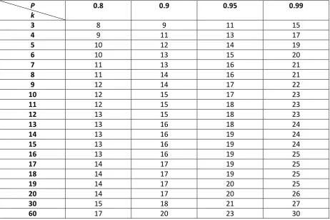
Using the expression (2.1.5), sample sizes are calculated for = 0.05, 0.01, P = 0.8, 0.9, 0.95, 0.99, = 0.3, 0.5 and k = 3(1)20, 30, 60 and are presented in Tables 3.1 through 3.4.

Table 3.1.





0.05,

 

0.5

P k

0.8 0.9 0.95 0.99

3 8 9 11 15

4 9 11 13 17

5 10 12 14 19

6 10 13 15 20

7 11 13 16 21

8 11 14 16 21

9 12 14 17 22

10 12 15 17 23

11 12 15 18 23

12 13 15 18 23

13 13 16 18 24

14 13 16 19 24

15 13 16 19 24

16 13 16 19 25

17 14 17 19 25

18 14 17 19 25

19 14 17 20 25

20 14 17 20 26

30 15 18 21 27

(5)

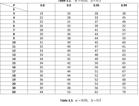
Table 3.2.





0.05,

 

0.3

P k

0.8 0.9 0.95 0.99

3 19 24 28 38

4 22 28 33 45

5 25 31 37 49

6 26 33 39 52

7 28 35 41 55

8 29 36 43 57

9 30 38 44 59

10 31 39 45 60

11 32 40 47 61

12 33 40 47 62

13 33 41 48 63

14 34 42 49 64

15 34 42 50 65

16 35 43 50 66

17 35 44 51 67

18 36 44 52 67

19 36 44 52 68

20 36 45 53 69

30 39 48 56 73

60 44 53 62 79

Table 3.3.





0.01,

 

0.5

P k

0.8 0.9 0.95 0.99

3 10 12 14 18

4 11 14 16 21

5 12 15 17 22

6 13 16 18 24

7 14 17 19 25

8 14 17 20 25

9 15 18 20 26

10 15 18 21 27

11 15 19 21 27

12 16 19 22 28

13 16 19 22 28

14 16 19 22 28

15 16 20 23 29

16 17 20 23 29

17 17 20 23 29

18 17 20 23 29

19 17 20 23 30

20 17 21 24 30

30 18 22 25 31

(6)

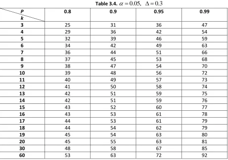
Table 3.4.





0.05,

 

0.3

P k

0.8 0.9 0.95 0.99

3 25 31 36 47

4 29 36 42 54

5 32 39 46 59

6 34 42 49 63

7 36 44 51 66

8 37 45 53 68

9 38 47 54 70

10 39 48 56 72

11 40 49 57 73

12 41 50 58 74

13 42 51 59 75

14 42 51 59 76

15 43 52 60 77

16 43 53 61 78

17 44 53 61 79

18 44 54 62 79

19 45 54 63 80

20 45 55 63 81

30 48 58 67 85

60 53 63 72 92

4. CONCLUDING REMARKS

Higher sample sizes are required for lower significance level , lower difference , higher power P and higher number of populations k.

(7)

5. REFERENCES

(1)Chow, S; Shao, J and Wang, H. (2008). “ Sample size calculations in clinical research”. Ed-2. Chapman & Hall / CRC, Biostatistics Series, pp.71.

(2)Nelson, P. R. (1983). “A comparison of sample sizes for the analysis of means and the analysis of variance”. Journal of Quality Technology 1, Vol. 15, pp. 33-39.

(3)Ott, E.R. (1967). “Analysis of means – a graphical procedure”. Industrial Quality Control 24, pp. 101-109.

(4)Rao, C. V and Harikrishna, S. (1997). “ A graphical method for testing the equality of several variances”. Journal of Applied Statistics 24, pp. 279-287.

(5)Wilson, E. B. and Hilferty, M. M. (1931). “ The distribution of chi-square,” Proceedings of National Academy of Sciences, U.S.A., 17.684.