Isolated Curves and the MOV Attack
Travis Scholl
October 11, 2017
Abstract
We present a variation on the CM method that produces elliptic curves over prime fields with nearly prime order that do not admit many efficiently computable isogenies. Assuming the Bateman-Horn conjecture, we prove that elliptic curves produced this way almost always have a large embedding degree, and thus are resistant to the MOV attack on the ECDLP.
1
Introduction
The security of elliptic curve cryptosystems is based on the difficulty of the elliptic curve discrete logarithm problem (ECDLP). For an elliptic curve E over a prime field Fp, the best known generic attack on the ECDLP takes roughly√poperations. Suppose that a new algorithmX was found that could solve the ECDLP on a subset W of elliptic curves overFp faster than all previously known algorithms. Given an instance of the ECDLP onE, if an attacker could construct an isogenyϕ:E→E0 withE0∈W, then they could transfer the instance toE0 where they could useX. The total time for this attack is bounded below by the timemthat it takes to computeϕ. Ifm≥√p, then this attack is no faster than generic algorithms, no matter how fast X is. LetT denote the set of curvesE0 such that an isogenyϕ:E→E0 can be computed in less than√ptime. We will assume that the probability that a random curve in T lies in W, is roughly the ratioof|W|to the number of elliptic curves overFp. For a randomE, we expect that|T | ≈√p, which in practice is≈2128. However, it is possible for|T |to be much smaller, so
thatE is resistant to this attack. For example, if≈2−50 and|T | ≤1000, then the probability
that the ECDLP onE can be efficiently transfered to someE0∈W is about 2−40. In this case,
we call Eisolated (a precise definition is given below). In this paper, we give an algorithm based on the complex multiplication (CM) method to generate isolated elliptic curves that are suitable for cryptography.
Remark 1.1. The hypothetical attack outlined above is motivated by the case of elliptic curves over composite degree extensions of prime fields (usuallyF2). In that case, Weil descent can
sometimes be used to solve the ECDLP significantly faster than generic methods on a small but non-negligible proportion of curves [25,26].
Theconductor gap (see Definition3.1) between two elliptic curves measures the difficulty of constructing an isogeny between them. If the conductor gap betweenE andE0 isL, then the fastest known algorithm for computing an isogeny betweenE andE0 takes roughlyL3 time. We
say an elliptic curveE is (L, T)-isolated if there are at most T curves whose conductor gap with E is at mostL. For example, ifEis (p1/6,1000)-isolated, then there are at most 1000 curvesE0 for which it would be feasible to construct an isogenyE→E0. ThusE is most likely resistant to the hypothetical attack described above.
main theorem shows that, under the Bateman-Horn conjecture, curves produced by our algorithm almost always have embedding degree larger than log2p.
Theorem 1.2. Assume the Bateman-Horn conjecture. There is an algorithm that takes as input a boundM, and returns an elliptic curveE over a prime fieldFp such that the following hold:
(i) M/2≤p≤M
(ii) #E(Fp) =rf wherer is prime andf |24
(iii) E is(p
p/50−100,8)-isolated.
The expected running time of the algorithm isO(log3M)multiplied by the time required to test
if an integer of size M is prime. IfM is sufficiently large, then the probability that the returned curve has an embedding degree less thanlog2p, is bounded above by
Clog
8
M
√
M
for some effectively computable constantC.
Remark 1.3. The Bateman-Horn conjecture is used to estimate how often several polynomials are simultaneously prime. While the conjecture gives an asymptotic formula for any collection of polynomials, we only require a big-Ω statement for how often three particular polynomials are simultaneously prime (see Problem6).
Remark 1.4. Experimentally, our algorithm works well whenM ≈2256. After several thousand
iterations, it never produced a curve with embedding degree>log2pand finished within the expected time (see Section6.4). However, we are unable prove an explicit lower bound for what “sufficiently large” is, nor can we give a computable upper bound for the implicit constant in the big-O notation for the run time. In Section6, we discuss these points as well as provide a reasonable assumption to solves these issues.
Theorem 1.2should be compared with the generic probability that a curve with prime order has embedding degree<log2p.
Theorem 1.5 (Balsubramanian and Koblitz [1, Thm. 2]). Let pbe a uniformly random prime in the interval[M/2, M], and E a random elliptic curve overFp of prime order. The probability that the embedding degree ofE is less than log2p, is bounded above by
Clog
9M
(log logM)2
M ,
for some effectively computable constantC.
Remark 1.6. When giving a conditional theorem in cryptography, it is important to avoid contrived conjectures that are custom built to fill gaps in security proofs [21], [19, Sec. 1.4.2]. The Bateman-Horn conjecture is of independent interest. It predates elliptic curve cryptography, and is a generalization of the well-known hypothesis H from Schinzel [32]. It is supported by substantial theoretical and numerical evidence. For this reason we feel that the use of the conjecture is justified.
1.1
Acknowledgments
I would like to thank my advisor Neal Koblitz for all of his support and guidance while working on this paper. I would also like to thank Bianca Viray for her patience in reading many first drafts, as well as David Jao for helpful conversations about computing isogenies between elliptic curves at a conference. Finally, I am grateful to my fellow graduate students for listening to me talk about elliptic curves in every seminar.
2
Background and Notation
LetE be an elliptic curve over a prime fieldFp. We will primarily consider primes on the order of 2256. LetN =|E(
Fp)|be the number of points, andt=p+ 1−N. Ift≡0 modpthenE is vulnerable to the MOV attack [27], so we will only consider the case whent6≡0 modp. In this caseEis called ordinary.
An isogeny is a surjective morphism of elliptic curves with finite kernel. The set of isogenies E→Edefined over the algebraic closureFpofFp, together with the 0 map form theendomophism ring EndE= EndFpE. IfE is ordinary then EndEis isomorphic to an order in an imaginary quadratic fieldK.
Let π ∈ EndE denote the Frobenius endomorphism, which on the level of points takes (x, y)7→(xp, yp). We identifyπwith an element ofK. Then trπ=tand Norm(π) =p[35, Ch. V]. This means that we can identify π= t+c
√ −d
2 , where−d= discK andc >0. Notice thatZ[π] is
the order inK of conductorc, and that
4p=t2+dc2. (1)
Given an elliptic curveE, there is an associated numberj(E) which determines the isomorphism type ofE overFp. j(E) is called thej-invariant of E. Throughout the rest of the paper, unless otherwise noted,E will represent an ordinary elliptic curve over the prime fieldFp.
2.1
Isogeny Classes
Definition 2.1. Theisogeny class IofE is the set of isomorphism classes (overFp) of elliptic curves that are isogeneous (overFp) toE.
The isogeny class ofE is uniquely determined byN = #E(Fp). This follows from Tate’s isogeny theorem, which says that two elliptic curves overFp are isogeneous if and only if they have the same number of points [35, Exercise. 5.4]. For every integerN in the Hasse interval [p+ 1−2√p, p+ 1 + 2√p], there is an elliptic curve with N points. Thus by Tate’s thereom, there are about 4√pisogeny classes. One can show using thej-invariant that there are roughly 2pisomorphism classes of elliptic curves over Fp. This means that on average, each isogeny class has about√p/2 curves.
An`-isogeny is an isogeny of degree`. We will only consider`-isogenies with`a prime other thanp. Such isogenies are separable and have a kernel of size`. Any separable isogeny between elliptic curves factors into a composition of isogenies of prime degree.
2.2
Endomorphism Classes
The isogeny classI ofEcan be partitioned into endomorphism classes. LetIO denote the set of curves inI whose endomorphism ring is isomorphic toO, an order in an imaginary quadratic field. We callIO theendomorphism class of Oin I.
Proposition 2.2. The endomorphism classes in I are precisely those associated to orders in the quadratic imaginary fieldQ(π)that contain Z[π]. For anyO ⊇Z[π], the size of IO is equal to the class numberh(O).
Endomorphism classes have O(√plogd) curves. To see this, letc0 be the conductor of an order appearing inI. Recall that the class number of an order of conductorc0 is approximately hc0 (see [9, Thm. 7.24] for a precise formula). The class number h is bounded above by
1
π
√
dlogd[6, Excercise 5.27b]. We also know thatc0 dividescbecause every order appearing in I contains the Frobenius ringZ[π]. It follows from (1) thathc0≤hc≤ πc
√
dlogd < 2
π
√
plogd. For a random curveEoverFpfor a random primep, we expect thatcis close to 1 [16, Sec. 6]. Because the endomorphism classes inI correspond to divisors of c, we do not expect to find many endomorphism classes. Thus on average, we should expect thatIEndE usually has roughly
√
pcurves.
2.3
Bateman-Horn Conjecture
We will be interested in how often several polynomials are simultaneously prime. For a single polynomial of degree one, we have the prime number theorem and Dirichlet’s theorem on primes in arithmetic progressions. Bateman and Horn made the following conjecture based on heuristics derived from the prime number theorem.
Definition 2.3. We say that a polynomial f ∈ Z[x] satisfies Bunyakovsky’s property if gcda∈Zf(a) = 1.
Warning 2.4. In order forfto satisfy Bunyakovsky’s property, it is necessary that the coefficients off are relatively prime. This condition is not sufficient, for example gcda∈Z(a
2+a) = 2.
Conjecture 2.5 (Bateman-Horn Conjecture [2]). Let f1, . . . , fk ∈Z[x] be distinct irreducible
polynomials such that their productQ
fi satisfies Bunyakovsky’s property. Let
Pf1,...,fk(N) ={a∈Z: 1≤a≤N andfi(a)is prime for alli= 1, . . . , k}.
Then
|Pf1,...,fk(N)| ∼ C D
N
logkN. (2)
Here D=Q
degfi,C=Q`prime
1−ω(`)/`
(1−1/`)k, andω(`)denotes the number of roots of Qf
i inF`.
Remark 2.6. There is a large amount of theoretical and numerical evidence for the Bateman-Horn conjecture. It reduces to Dirichlet’s theorem on primes in arithmetic progressions for a single polynomial of degree 1. It also agrees with the twin prime conjecture and the Sophie Germain prime conjecture [34, Ch. 5.5]. More recently, an analog of the conjecture has been proven for function fields [10].
2.4
The MOV Attack
The MOV attack transfers a discrete log fromE(Fp) toF×pk for some positive integerk. The idea is to leverage sub-exponential time algorithms for solving discrete logs in the multiplicative group of a finite field. A necessary condition for this transfer is that|E(Fp)|dividespk−1. The smallest possiblekis called theembedding degree1 ofE. This is the same as the multiplicative order of p
in (Z/NZ)× whereN =|E(Fp)|. For more on the MOV attack see [27]2or [35, Ch. XI.6]. Ifk >log2p, then the MOV attack will not be faster than trying to solve the discrete log on E directly [1]. Therefore we are primarily interested in curves with embedding degree>log2p.
1
The embedding degree may also refer to the multiplicative order ofpin (Z/rZ)×whereris the largest prime
factor ofN. This is because cryptosystems are usually constructed using the largest prime order subgroup of the elliptic curve group, rather than the entire group. We will only be interested in curves with nearly prime order, so the difference between usingN orris not important. Also implicitly we are avoiding anomalous curves whereN=p, i.e.
t= 1. Anomalous curves are extremely rare but should be avoided as there are known attacks against them [36].
2Technically, the attack of [27] requires thatN be relatively prime top−1. But, if this is not the case then there is
an attack described by Frey and R¨uck [12] which also transfers the ECDLP toF×pk. We will not differentiate between
3
Isolated Curves
Definition 3.1. The conductor gap of two orders in a fixed quadratic imaginary field is the largest prime dividing the conductor of one and not the other. The conductor gap between two isogenous elliptic curves is defined to be the conductor gap of their endomorphism rings. If the curves are not isogeneous, then their conductor gap is∞. TheL-conductor-gap classof a curve E is the set of all curvesE0 such that the conductor gap betweenE andE0 is less thanL.
Proposition 3.2. Let ϕ : E → E0 be an `-isogeny for some prime `. If O and O0 are the endomorphism rings ofE andE0 respectively, then one of the following holds:
[O:O0] =`, [O0:O] =`, O=O0.
Proof. [22, Prop. 21].
In the first two cases of Proposition3.2, we say that ϕisvertical; otherwiseϕishorizontal. Horizontal isogenies stay inside the same endomorphism class while vertical ones move to a new class. The main implication of Proposition3.2 is that if two endomorphism classes have conductor gap a prime`, then any isogeny between them factors through an`-isogeny. Unless otherwise noted, throughout the rest of the paper`will denote a prime not equal top.
Definition 3.3. Let E be an elliptic curve overFp. We will sayE isisolated with gapL and set-sizeT, or (L, T)-isolated, if theL-conductor-gap class ofEhas at mostT curves.
Remark 3.4. The observation that isolated curves are resistant to isogeny based attacks has been noted before in the literature. This idea is discussed in [20, Sec.11.2], [17, Sec. 7.1], and [25, Rem. 6]. This idea has also been applied to Jacobians of curves of genus 2 [39].
3.1
Computational Complexity of Isogenies
The computational complexity of an isogeny depends on its degree, but the complexity is different for horizontal and vertical isogenies. The fastest known method [22] for constructing a vertical isogeny fromEinvolves constructing the modular polynomial Φ`. Finding Φ` modpis the most expensive step and the best known methods takeOe(`3) time andOe(`2) space [4] (recall that
e
O(f) meansO(flogkf) for some integerk). Φ`is a polynomial of degree`+ 1 in two variables, so any method which involves computing Φ` must take Ω(`) time and space. Moreover, because we represent`-isogenies using either polynomials of degree`, or a list of points in the kernel; any algorithm which computes an`-isogeny will need at least Ω(`) space.
For horizontal isogenies where the endomorphism ring has a small discriminant, there are much faster algorithms which are polynomial in log` [3,18]. These methods do not extend to vertical isogenies crossing a large conductor gap. Therefore we can only effectively transport the ECDLP to another endomorphism class when the conductor gap is less thanp1/6.
The best algorithm known for solving the ECDLP on a general elliptic curve takesOe(
√
p) time [28]. If ` ≥p1/6, then computing a vertical`-isogeny takes similar time to solving the
ECDLP. If two endomorphism classes have a conductor gap of at leastp1/6, then there is no
significant benefit in transferring the ECDLP across the gap.
3.2
Examples
Example 3.5. LetEbe the elliptic curvey2=x3+6xover
Fpwherep= 12475737285765000161≈ 263.4. Note that EndE ∼=
Z[i] has class number 1, so E is the only curve in its
endomor-phism class. The Frobenius endomorendomor-phism π generates an orderZ[π] with prime conductor
c= 2559154831≈231.2. This means that the isogeny class ofE has two endomorphism classes:
One which contains onlyE, and another which containsh(Z[π]) = 1279577416≈230.2 curves.
Example 3.6. Let E be the elliptic curvey2 =x3+ 350xover
Fp wherep= 122501. As in the previous example, the endomorphism class ofE has only one curve. However, in this case
Z[π] has conductor 1, so the isogeny class ofE contains onlyE, and Eis (∞,1)-isolated. This
example is highly atypical because the tracet= 700 = 2√p
is at the extreme end of the Hasse bound.
4
Generating Isolated Curves
In this section we give an algorithm to generate isolated elliptic curves. We will apply some slight modifications to the algorithm presented here in order to prove Theorem1.2. For use in cryptography, we would like to generate prime ordered curves. However there are some basic obstructions to a curve having prime order. For example, consider equation1. In order forpto be an odd prime, ifdis even thent must be even. It follows thatN =p+ 1−t is also even. In this case, the choice ofdforced a factor of 2 to divide N. Fortunately, the only obstructions to N being prime are a few factors of 2 and 3.
For any integera≡0,3,4 mod 8, define3thecofactor to be
cofa= 2ν2·3ν3, (3)
where
ν2=
0 ifa≡3,11,19,27 mod 32 1 ifa≡4,8,20,24 mod 32 2 ifa≡0,12,16 mod 32 3 ifa≡28 mod 32,
ν3=
(
0 ifa6≡2 mod 3 1 ifa≡2 mod 3.
Algorithm 1
Isolated Curve
Input:
a positive integer
M
and fundamental discriminant
−
d <
0.
Output:
an elliptic curve defined over
F
pwhere
dM16< p <
dM41:
repeat
steps 2-5
2:
t
←
random integer in
h
−
√
M ,
√
M
i
\ {
0
,
1
,
2
}
3:
c
←
random integer in
h
√M 2
,
√
M
i
4:
p
←
t2+dc4 2 5:N
←
p
+ 1
−
t
6:
until
p
,
N/
cof
dc2are integers and
p, c, N/
cof
dc2are prime
7:
j
←
root of the Hilbert class polynomial for
Q(
√
−
d
) mod
p
8:
E
←
elliptic curve over
F
pwith
j
(
E
) =
j
and
|
E
(
F
p)
|
=
N
9:
return
E
Remark 4.1. Algorithm1is not optimized for efficiency. For example, if d≡0 mod 4 thent must be even. Thus by choosing only even values oft in step 2, we expect the runtime to be reduced by a factor of 2. We present the unoptimized version for simplicity.
Remark 4.2. The reason for removing 0,1,2 from possible values oft is to avoid the attacks described in [36], [27], and [12].
3
The value of cofawas calculated by considering the equation 4N= (t−2)2+amodulo powers of 2 and 3. Herea
Remark 4.3. One drawback4 of using the CM method is that we do not have full control over
the primep. That is, we can not choose parbitrarily and then construct an isolated curve over
Fp. This makes it more difficult to find pwith special properties, such as a small Hamming weight (which can lead to more efficient implementations). However, we can lower the Hamming weight ofpwith the following modifications. Instead of choosingcrandomly, fixc to be a large prime of small Hamming weight. Also, restrict the search fortto integers with small Hamming weight. Becausepis given by a simple expression intandc, the resulting value ofpwill likely have small Hamming weight.
First we will explain the last steps of the algorithm. The following facts are the basis of the well known CM method [7, Ch. 18.1]:
(i) The Hilbert class polynomial ofK=Q(
√
−d) has a root in Fp by construction.
(ii) There exists an elliptic curveE/FpwithN points andj(E) =j.
An efficient algorithm for findingE, givenj andN can be found in [31]. Sincej(E) is a root of the Hilbert class polynomial modp, it follows that EndE∼=OK [37, Sec. 2.8]. If the choice ofd is bounded by a constant, then steps 7 and 8 in the algorithm have a running time ofO(1). The main factor in the running time comes from the loop in steps 2 through 5.
Proposition 4.4. If the main loop of Algorithm1 terminates, then the curve E returned by the algorithm is isolated with gap
√ M
2 and set-size 1
π
√
dlogd.
Proof. We are assumingp, c, N/cofdc2 are prime and we want to show thatE is isolated. Let K=Q(
√
−d). By the explanation above, EndE∼=OK. Letπ∈EndE denote the Frobenius endomorphism ofE. InOK,πcorresponds (up to conjugation) to t+c
√ −d
2 . We also know that
c= [OK :Z[π]]. Becausec was chosen to be prime, there are two endomorphism classes in the
isogeny class of E corresponding to OK and Z[π]. The endomorphism class of OK contains h(OK)≤ π1
√
dlogdcurves. Therefore,Eis isolated with gapc≥ √
M
2 and set-size 1
π
√
dlogd.
Remark 4.5. It is easy to alter Algorithm1 to produce curves that are (∞,1)-isolated, meaning that the entire isogeny class contains a single curve, similar to Example 3.6. To do this, we choosedsuch thatQ(
√
−d) has class number 1, and fixc= 1. However, we do not know how to prove that curves generated this way usually have an embedding degree>log2p. This is because
there are too few values oft such thatpandN/cofd are simultaneously prime. Even though the Bateman-Horn conjecture gives an asymptotic formula, it is not enough to prove a bound on the embedding degree using the methods in Section5. Moreover, due to their rarity, one could argue that (∞,1)-isolated curves are too special for cryptography, and that there may not be sufficient randomness in their selection.
5
Improbability of the MOV Attack on Isolated Curves
5.1
Notation
In [1], Balasubramanian and Koblitz proved that a random prime order elliptic curve over a random prime field almost always has a large embedding degree. Their work has been extended in several ways [8,24]. We want to emulate the main theorem of [1] for isolated curves. The main difference is that in [1], the authors were able to vary the prime and the number of points subject only to the Hasse bound. There is less flexibility in our case due to restrictions on the conductorcand the discriminantd.
We will use the following notation:
−d= fixed small (<100) fundamental discriminant of a quadratic imaginary field
p=p(t, c) = t
2+dc2
4 , N =N(t, c) =p+ 1−t,
cof = cof(c) = cofcd2 as defined inSection 4, r=r(t, c) = N cof.
Remark 5.1. Note thatrisnota polynomial int, cbecause cof(c) depends only on the valuation ofdc2 at 2 and 3. We will apply a linear change of variables incin order to fix the cofactor.
Define the following sets:
SM = n
(t, c)∈h1,√Mi×h√M /2,√Mi:p, r, care primeo
SM,K = n
(t, c)∈SM: the order ofpin (Z/rZ)× is at mostK
o
SM(t) ={c: (t, c)∈SM}
SM,K(t) ={c∈SM(t) : (t, c)∈SM,K}.
SM represents possible pairs t, cthat Algorithm1could use to generate an isolated curve. In particular, the expected number of pairst, csampled by Algorithm1is |SM|
M . SM,K represents those pairs which result in a curve with embedding degree at most K. SM(t) andSM,K(t) represent pairs with a fixedtvalue.
5.2
Main Results
Our goal for this section is to find an upper bound for SM,K(t0)
SM(t0) for a fixed integert0. This is roughly the probability that Algorithm1returns a curve with embedding degree at most K given thatt=t0.
First we give an upper bound forSM,K(t0).
Proposition 5.2. Let K, M be any positive integers. Then there is a universal constant A1
such that for any integer t0 with |t0|>1,
|SM,K(t0)|<A1K2log|t0|.
Proof. LetLk=
primes`:`|(t0−1)k−1 . By constructionr|pk−1⇔r|(p−N)k−1 =
(t0−1)k−1. Hence there is a mapϕ:SM,K(t0)→
SK
k=1Lk given byc7→r(t0, c).
Next we will show that|ϕ−1(`)| ≤16. Note thatN(t
0, c) is a quadratic polynomial inc, so
there are at most 2 values ofcsuch thatN(t0, c) is the same. There are 8 possible values of cofc, hence there are at most 16 values ofcwhich could give the same value of r(t0, c). Therefore
|SM,K(t0)|=
ϕ−1 K [ k=1 Lk ! ≤16 K [ k=1 Lk .
It remains to bound theLk. The number of prime divisors of (t0−1)k−1 is bounded by
log2|t0−1|k≤klog2(|t0|+ 1). Hence
K [ k=1 Lk ≤ K X k=1
|Lk| ≤
K X
k=1
klog2(|t0|+ 1) =
K(K+ 1)
2 log2(|t0|+ 1)≤2.4K2log(|t0|).
The last inequality holds for all|t0| ≥2, so we may takeA1= 2.4.
Next we will to bound SM(t0) from below. Becauset0is fixed, we will be able to apply the
Bateman-Horn conjecture. However, in order to apply the conjecture, we first need a change of coordinates which makespand rinto polynomials satisfying Bunyakovsky’s property.
Lemma 5.3. Let−dbe a fundamental discriminant for a quadratic imaginary field such that d <100. Then there are computable constantsm1, b1, m2, b2∈Z≥0, such that the linear change
(i) fd(c0)2 is constant as a function ofc.
(ii) p0 =p(t0, c0)andr0=r(t0, c0)are integer polynomials in t andc.
(iii) For any t ∈ Z, the product p0·r0·c0/gcd(m2, b2) satisfies Bunyakovsky’s property as a
polynomial inc.
Remark 5.4. In condition (iii) of Lemma 5.3, we include c0/gcd(m2, b2) rather than just c0
because of the cased≡7 mod 8. In this case,p= t2+dc2
4 is an odd integer only iftandc are
even. In particular, we cannot have bothc0 andp0 simultaneously prime whend≡7 mod 8.
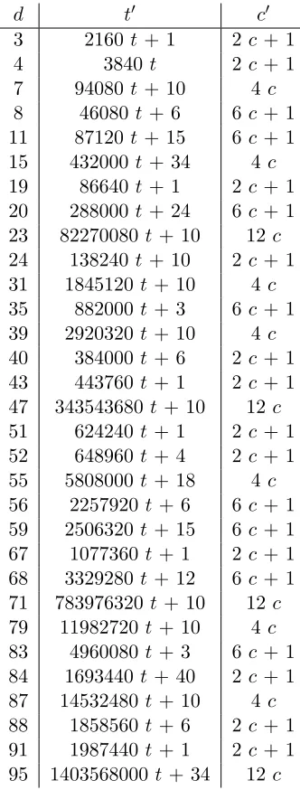
Proof of Lemma 5.3. We will prove the claim in detail for d= 4 by showing t0 = 3840t and c0 = 2c+ 1 satisfy properties (i)-(iii). The other cases are similar, and the corresponding change of coordinates are given in Table1.
(i) For anyc, we have thatd(c0)2≡4 mod 32 and d(c0)26≡2 mod 3. Hence cof
d(c0)2 = 2 for allc.
(ii) To showp0 andr0 are integer polynomials, we just have to expand out the definitions:
p0=p(t0, c0) = 3686400t2+ 4c2+ 4c+ 1
r0=r(t0, c0) =N(t0, c0)/2 = 1843200t2+ 2c2−1920t+ 2c+ 1.
(iii) Letg(t, c) =p0·r0·c0 ∈Z[t, c] andt0∈Z. To show thatg(t0, c)∈Z[c] satisfies Bunyakovsky’s
property, it is sufficient to check that gcd{g(t0,0), . . . , g(t0,5)}= 1 asg(t0, c) is a degree 5
polynomial inc.5
A direct computation6 shows that
3g(t,0) + 4g(t,1) + 17g(t,2)−36g(t,3) + 23g(t,4)−5g(t,5) = 960.
Therefore
gcd{g(t0,0), . . . , g(t0,5)}= gcd{g(t0,0), . . . , g(t0,5),960}
= gcd{g(0,0), g(0,1), . . . , g(0,5)} = 1.
The second to last equality follows from the fact that t0 ≡0 mod 960 by construction. The last equality follows from the fact thatg(0,0) = 1.
Remark 5.5. We expect Lemma 5.3to hold for alldwith many different possibilities formi, bi.
Proposition 5.6. Assume the Bateman-Horn conjecture and that d <100 andd6≡7 mod 8. Letm1, b1 be the constants from Lemma 5.3. For any integert0, there are constants A2,B2 such
that for all M >B2,
|SM(m1t0+b1)|>A2
√
M log3M.
The constantsA2,B2 depend ont0. Moreover, the constantA2 is effectively computable.
Proof. Lett0(t) =m1t+b1andc0(c) =m2c+b2be the change of coordinates given by Lemma5.3.
Then p0 =p(t0(t0), c0), r0 = r(t0(t0), c0), andc0 are integer polynomials in Z[t, c], and satisfy
Bunyakovsky’s property. Moreover, p0 and r0 are irreducible because their roots are linear combinations of the roots ofp(t0, c), N(t0, c) respectively. The latter are complex as long as
5
This condition is also sufficient, see [5, Exercise 1.3].
6This computation was done by constructing the matrix with rows given by the coefficients of theg(t, i), and then
d
t
0c
03
2160
t
+ 1
2
c
+ 1
4
3840
t
2
c
+ 1
7
94080
t
+ 10
4
c
8
46080
t
+ 6
6
c
+ 1
11
87120
t
+ 15
6
c
+ 1
15
432000
t
+ 34
4
c
19
86640
t
+ 1
2
c
+ 1
20
288000
t
+ 24
6
c
+ 1
23
82270080
t
+ 10
12
c
24
138240
t
+ 10
2
c
+ 1
31
1845120
t
+ 10
4
c
35
882000
t
+ 3
6
c
+ 1
39
2920320
t
+ 10
4
c
40
384000
t
+ 6
2
c
+ 1
43
443760
t
+ 1
2
c
+ 1
47
343543680
t
+ 10
12
c
51
624240
t
+ 1
2
c
+ 1
52
648960
t
+ 4
2
c
+ 1
55
5808000
t
+ 18
4
c
56
2257920
t
+ 6
6
c
+ 1
59
2506320
t
+ 15
6
c
+ 1
67
1077360
t
+ 1
2
c
+ 1
68
3329280
t
+ 12
6
c
+ 1
71
783976320
t
+ 10
12
c
79
11982720
t
+ 10
4
c
83
4960080
t
+ 3
6
c
+ 1
84
1693440
t
+ 40
2
c
+ 1
87
14532480
t
+ 10
4
c
88
1858560
t
+ 6
2
c
+ 1
91
1987440
t
+ 1
2
c
+ 1
95
1403568000
t
+ 34
12
c
t0(t0) 6= 0,2. Thus p0, r0, and c0 satisfy the hypothesis of the Bateman-Horn conjecture as
polynomials inZ[c].
LetSM0 (t0) denote the set ofc0 such thatc0(c0)∈SM(t0(t0)), and
Pp0,r0,c0(
√
M) =nc0∈[1,
√
M] :p0(c0),r0(c0), andc0(c0) are prime
o .
By above, we can apply the Bateman-Horn conjecture to the polynomialsp0,r0, andc0. This means that there is a constant C, depending on the polynomialsp0, r0, andc0 (which depend only ondandt0), such that
Pp0,r0,c0(
√
M) ∼ C
√
M log3√M.
Notice thatSM0 (t0) =Pp0,r0,c0(
√
M)∩J(√M) where J(M) = [ 1
m1(
1 2
√
M −b1),m11(
√
M−b1)].
We will assumeM max{m2
1,16b21}so that
|S0M(t0)|=
P 1 m1 1 2 √
M −b1
− P 1 m1 √ M −b1
∼ C
1
m1(
1 2
√
M −b1))
log3 1
m1(
1 2
√
M −b1))
− C
1
m(
√
M−b1))
log3 1
m1( √
M−b1))
≥ C 2m1
√
M−2b1
log3M
> C 4m1
√
M
log3M.
Thus there is some constant B2such that|SM0 (t0)|>4mC1
√ M
log3M for allM >B2. Note that the
constant B2 depends on t0. The mapc07→c0(c0) gives us an inclusion SM0 (t0),→SM(t0(t0)).
Therefore the inequality in the claim holds withA2= 4mC
1.
It remains to show that the constantCgiven in the Bateman-Horn conjecture is computable.7
Let
g1=t20+dc 2, g
2= (t0−2)2+dc2, g3=c, and G=g1·g2·g3.
Define ωi(p) to be the number of roots ofgi modpandω(p) to be the number of roots ofG modp. ThenGdiffers fromp0·r0·c0 by a linear change of coordinates and scaling. It follows that the constantC differs from the product
C2=
Y
p≥5
1−ω(p)/p (1−1/p)3
in at most a finite number of factors. So it is sufficient to showC2is computable. Notice that for
any primep≥5:
g1(c)≡g2(c)≡0 modp ⇒ p|t0+ 2,
g1(c)≡g3(c)≡0 modp ⇒ p|t0,
g2(c)≡g3(c)≡0 modp ⇒ p|t0−2.
LetS denote the set of primes dividing 6dt0(t0−2)(t0+ 2). Then for any primep6∈S,
ω(p) =ω1(p) +ω2(p) +ω3(p).
7The proof of convergence for the constant in the Bateman-Horn conjecture only relies on the Chebotarev density
Letχ(p) = 1 if−dis a square modpand−1 otherwise. Then one can show that for anyp6∈S we have that
ω1(p) =ω2(p) =χ(p) + 1
therefore
ω(p) = 2(χ(p) + 1) + 1.
Note that the product
Y
p
1−(2(χ(p) + 1) + 1)/p (1−1/p)3 =C3
Y
p
1−χ(p)
p 2
where C3 is an effectively computable constant. By Dirichlet’s analytic formula,
Y
p
1−χ(p)
p 2
= k √
d 2πh
!2
where k,hare the number of roots of unity and class number ofQ(
√
−d) respectively.
Theorem 5.7. Assume the Bateman-Horn conjecture and that d < 100, and suppose d6≡7 mod 8. Let m1, b1 be the constants from Lemma 5.3, which depend only on d. For any fixed
integert0, there are constants A3,B3 such that the probability thatc∈SM,K(m1t0+b1)given
thatc∈SM(m1t0+b1)is bounded above by
A3
K2log4
M
√
M
for allM >B3. The constantA3 is computable.
Proof. We have to bound SM,K(m1t0+b1)
SM(m1t0+b1) above. This follows immediately from the previous propositions. Proposition5.2 gives an upper bound forSM,K(m1t0+b1), and Proposition5.6
gives a lower bound forSM(m1t0+b1).
Warning 5.8. We do not have a computable upper bound for the constant B3.
5.3
Proof of the Theorem
1.2
Algorithm 2
Isolated Curve
Input:
positive integer
M
Output:
isolated (with gap
p
p/
50
−
100 and set-size 8) elliptic curve defined
over
F
pwith
M/
2
≤
p
≤
M
.
1:
−
d
←
fundamental discriminant such that 1
≤
d
≤
100 and
d
6≡
7 mod 8
2:
m
1, b
1, m
2, b
2←
constants from Lemma
5.3
3:
t
←
integer such that 3
≤
t
≤
100 and
t
≡
b
1mod
m
14:
repeat
steps 5-7
5:
c
←
random integer in
h
p
(2
M
−
t
2)
/d,
p
(4
M
−
t
2)
/d
i
with
c
≡
b
2mod
m
26:
p
←
t2+dc4 2 7:N
←
p
+ 1
−
t
8:
until
p
,
c
, and
N/
cof(
dc
2) are prime
9:
j
←
root of the Hilbert class polynomial for
Q(
√
−
d
) mod
p
10:
E
←
elliptic curve over
F
pwith
j
(
E
) =
j
and
|
E
(
F
p)
|
=
N
11:
return
E
Proof of Theorem 1.2. We will show that Algorithm2 satisfies the claims in Theorem1.2. By the Bateman-Horn conjecture and Lemma5.3, for any fixedd, tas chosen in the algorithm, the number of possible values ofc≤√M such thatp, c, N/cof(dc2) are simultaneously prime, is
Ω√M /log3M. Because there is a finite number of possibilities fort, d, which are independent ofM, this implies that the expected number of iterations of the main loop of Algorithm2is O log3M
.
The probability that the embedding degree of the returned curve is less than log2pfollows from Theorem 5.7 using K = log2M. Note that here we are using that t, d are bounded
independently of M, in order to average the result of Theorem 5.7 for all values of t in the interval [3,100].
The resulting curve E has N points, whereN =r·cof(dc2) and r is prime. Recall that
cof(dc2)|24 by definition (see Equation3). Also,E is isolated with gapc and set-size 8 because
cis prime, and the boundd≤100 implies that the class number ofQ(
√
−d) is at most 8. The lower boundc≥p
p/50−100 follows from a straightforward computation.
Remark 5.9. The bound ontin Algorithm 2is mostly arbitrary. It is important that the upper bound on|t|is independent ofM. The lower boundt≥3 is for the same reason as the restriction ontin Algorithm1.
6
Extending the Results
The goal of this section is to discuss the following issues with Theorem 1.2:
• The algorithm used in the proof (Algorithm2) places a restriction ont, limiting the amount of randomness in the selection of an isolated curve.
• It does not give a computable bound lower bound for what “sufficiently large” is.
Recall that the main idea of both Algorithm 1and Algorithm2 is to search for integerst, c such that three functions (p(t, c),r(t, c) andc) are simultaneously prime. Algorithm2imposes a restriction ontthat allowed us to reduce to the one variable case and apply the Bateman-Horn conjecture. We expect that the restriction ont is unnecessary, and that the following properties hold:
(ii) The probability that a curve returned by Algorithm1has an embedding degree <log2M isOlog√8M
M
.
(iii) The implied constants in these estimates are computable.
In the notation of Section5, all three properties reduce to giving computable bounds forSM and SM,K. Recall that the expected number of iterations of the main loop of Algorithm1is roughly
|SM|
M and the probability of an embedding degree less thanK is about |SM,K|
|SM| . For Theorem1.2, we fixed t and gave bounds for SM,K(t) and SM(t) in Proposition 5.2 and Proposition 5.6 respectively. We would like to extend those bounds toSM,K andSM.
Proposition 6.1. There is a computable constantA4 such that for any positive integersM and
K,
|SM,K| ≤ A4K2
√
MlogM.
Proof. By definition|SM,K| ≤P √
M
t=1 |SM,K(t)|. Then by Proposition5.2,
|SM,K| ≤ √
M X
t=1
A1K2logt≤ A1K2
√
Mlog√M ,
where A1is the constant from Proposition5.2. Hence we may takeA4=A12 .
Problem. Find a computable numberA5, depending only on the fundamental discriminantd,
such that for any positive integerM,
|SM|>A5
M log3M.
Remark 6.2. A solution to Problem6 would be useless in practice ifA5 is too small (e.g. 2−100).
Hence we implicitly require thatA5lies within a reasonable range, such asA5>2−20.
6.1
An Alternative Conjecture
Even under the Bateman-Horn conjecture we are unable to solve Problem 6. This is because the Bateman-Horn conjecture only gives an asymptotic formula; it does not provide information about the error term.8 However, there is another natural conjecture one may consider related to
the Bateman-Horn conjecture.
Conjecture 6.3. Letf1, . . . , fk ∈Z[x, y]be such that everyfiis irreducible andgcda,b∈Z
Q
fi(a, b) = 1. LetPf1,...,fk(N)denote the number of pairsa, bsuch that0≤a, b≤N andf1(a, b), . . . , fk(a, b) are simultaneously prime. Then for anyN0>0, there exists a computable constantC(depending
onN0 and thefi) such that
Pf1,...,fk(N)> C N2
logkN for allN > N0.
Remark 6.4. As stated, the constant C in Conjecture 6.3 depends on N0. We could have
equivalently stated the conjecture withCindependent ofN0. However, in practice we usually
avoid small values ofN.
Recall that before the prime number theorem was proven, Chebyshev showed thatπ(N)≥
log 2 2
N
logN for all N ≥ 2 [34, Thm. 5.3]. In a way, Conjecture 6.3 is to the Bateman-Horn conjecture as Chebyshev’s inequality is to the prime number theorem. Conjecture6.3is weaker than the Bateman-Horn conjecture in the sense that it only asks for a lower bound, not an asymptotic formula. In fact, Conjecture6.3would follow from the Bateman-Horn conjecture if it had included a clause about the error term.
8
6.2
Heuristic Evidence
The same heuristics used to justify the Bateman-Horn conjecture suggest that Pf1,...,fk in Conjecture6.3has the right order of magnitude. Letf(x, y)∈Z[x, y] such that gcdx,y∈Zf(x, y) =
1. If we pretend that f(x, y) acts like a random number, then the probability that f(x, y) is prime should be roughly 1
log|f(x,y)|. Ifx, yare chosen independently from a uniform distribution on [0, N], then the probability that f(x, y) is prime should be roughly 1
dlogN whered is the degree off (i.e. the highest total degree of any monomial inf). Given multiple polynomials f1, . . . , fk satisfying the hypothesis in Conjecture6.3, we expect that the probability that they are simultaneously prime is the product of the probabilities for eachfi, up to some constant correction factor. This suggests thatPf1,...,fk = Θ
N2
logkN
, but gives no insight into the constants.
6.3
Theoretical Evidence
Conjecture6.3also differs from the Bateman-Horn conjecture in that it applies to polynomials in two variables. There are many cases where the conjecture can be proven. For example, we can apply the prime number theorem for quadratic fields to estimate how often certain quadratic forms are prime [15, Thm. 21.1]. The Friedlander-Iwaniec theorem [14] gives an asymptotic density of primes of the form x2+y4. More recently considered were pairs x, y such that x2−xy+y2 and 2x−y are both prime [29]. One the examples closest to Problem 6is the
following result of Fouvry and Iwaniec.
Theorem 6.5 (Fouvry and Iwaniec [15, Thm. 20.3], [11]). LetΛ be the von Mangoldt function defined by
Λ(n) = (
logp ifn=pk for some primep 0 otherwise.
Then
X
x2+y2≤N
Λ(x)Λ(x2+y2) =πH 4 N+O
N
log1/4N
where the sum is over positive integer, H=Q p
1−χp−(p1), and
χ(p) =
1 p≡1 mod 4 −1 p≡3 mod 3 0 p= 2.
Corollary 6.6. LetPx,x2+y2(N)denote the number of pairsx, y∈[0, N]such thatxandx2+y2 are simultaneously prime. Then
Px,x2+y2(N) = Ω N2
log2N
.
Proof. First notice that
Px,x2+y2(N) =
X
x,x2+y2prime
0<x,y<N 1
≥ X
x,x2+y2prime
0<x2+y2<N2 1
≥ 1 2 log2N
X
x,x2+y2prime
0<x2+y2<N2
The only difference between the last sum and the sum in Theorem6.5, is that the latter includes prime powers. The number of prime powers less thanN2is bounded above by log(N)π(N)<2N.
For each prime powerpk less thanN, there are at most 4(k+ 1) pairsx, ysuch thatx2+y2=pk. This is because there are at most k+ 1 ideals inZ[i] with norm pk, and each has at most 4
distinct generators. Therefore
Px,x2+y2(N)≥ 1 2 log2N
X
x2+y2≤N2
Λ(x)Λ(x2+y2)− 4N logN.
The claim now follows from Theorem 6.5.
If we restrict to even values of t, then ford= 4 we have thatp(t, c) = t
2
2
+c2. Hence the corollary above implies that ford= 4 we have
#
t, c:p=t
2+dc2
4 andcare prime andp≤M
= Ω
M
log2M
.
This agrees with our heuristics because we have two polynomials and the probability both are prime is roughly 1
log2M when choosingt, crandomly in [0, √
M]. We expect the same principal term for other values of d. Furthermore, adding the requirement that r(t, c) is prime should change the principle term by a factor of 1
logM. It is unclear if the methods used in the proof of Theorem6.5could extend to cover pairs t, csuch that all three functionsp, r, andc are all simultaneously prime.
6.4
Numerical Evidence
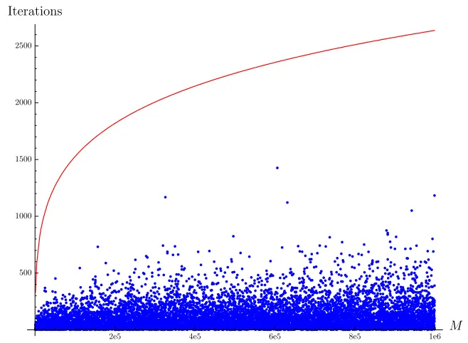
We implemented Algorithm1withd= 4 using a few modifications for efficiency, such as only choosing odd values ofcand even values oft. For a few values ofM, we counted the number of iterations the main loop ran until the algorithm returned. Equivalently, this is the number of pairst, cchosen at random untilp,r, andcwere simultaneously prime. The number of iterations was always below log3M as shown in Figure1.
We also computed the embedding degree of a curve returned by Algorithm1 withM = 298.
In 10000 runs we observed 0 curves with embedding degree<log2(M). This should be compared with the bound log√8(M)
M ≈0.80527.
7
Conclusion
We acknowledge that a solution to Problem 6may not be as mathematically interesting as proving an asymptotic formula with an optimal error bound for a generalized, two variable Bateman-Horn conjecture. However, a solution to Problem6would be enough to:
(i) Prove the efficiency of an algorithm to generate an isolated curve with large embedding degree.
(ii) Prove that the space of isolated curves is large enough to provide sufficient randomness in parameter selection.
These facts are enough to show that isolated curves provide cryptosystems resistant to the isogeny based attacks described in the introduction.
References
2e5 4e5 6e5 8e5 1e6 M 500
1000 1500 2000 2500
Iterations
Figure 1: Comparing the observed number of samples of
t, c
used in Algorithm
1
with log
3M
for
various values of
M
.
[2] P. T. Bateman and R. A. Horn. A heuristic asymptotic formula concerning the distribution of prime numbers. Math. Comp., 16:363–367, 1962.
[3] R. Br¨oker, D. Charles, and K. Lauter. Evaluating large degree isogenies and applications to pairing based cryptography. InPairing-based cryptography—Pairing 2008, volume 5209 of LNCS, pages 100–112. Springer, Berlin, 2008.
[4] R. Br¨oker, K. Lauter, and A. V. Sutherland. Modular polynomials via isogeny volcanoes. Math. Comp., 81(278):1201–1231, 2012.
[5] P.-J. Cahen and J.-L. Chabert. Integer-valued polynomials, volume 48 ofMathematical Surveys and Monographs. American Mathematical Society, Providence, RI, 1997.
[6] H. Cohen. A course in computational algebraic number theory, volume 138 ofGraduate Texts in Mathematics. Springer-Verlag, Berlin, 1993.
[7] H. Cohen, G. Frey, R. Avanzi, C. Doche, T. Lange, K. Nguyen, and F. Vercauteren, editors. Handbook of elliptic and hyperelliptic curve cryptography. Discrete Mathematics and its Applications (Boca Raton). Chapman & Hall/CRC, Boca Raton, FL, 2006.
[8] A. C. Cojocaru and I. E. Shparlinski. On the embedding degree of reductions of an elliptic curve. Inform. Process. Lett., 109(13):652–654, 2009.
[9] D. A. Cox.Primes of the formx2+ny2: Fermat, class field theory, and complex multiplication.
Pure and Applied Mathematics (Hoboken). John Wiley & Sons, Inc., Hoboken, NJ, second edition, 2013.
[10] A. Entin. On the Bateman-Horn conjecture for polynomials over large finite fields. ArXiv e-prints, Sept. 2014. http://arxiv.org/abs/1409.0846.
[11] E. Fouvry and H. Iwaniec. Gaussian primes. Acta Arith., 79(3):249–287, 1997.
[12] G. Frey, M. M¨uller, and H.-G. R¨uck. The Tate pairing and the discrete logarithm applied to elliptic curve cryptosystems. IEEE Trans. Inform. Theory, 45(5):1717–1719, 1999. [13] J. Friedlander and A. Granville. Limitations to the equi-distribution of primes. IV. Proc.
[14] J. Friedlander and H. Iwaniec. Using a parity-sensitive sieve to count prime values of a polynomial. Proc. Nat. Acad. Sci. U.S.A., 94(4):1054–1058, 1997.
[15] J. Friedlander and H. Iwaniec.Opera de cribro, volume 57 ofAmerican Mathematical Society Colloquium Publications. American Mathematical Society, Providence, RI, 2010.
[16] D. Jao, S. D. Miller, and R. Venkatesan. Do all elliptic curves of the same order have the same difficulty of discrete log? InAdvances in cryptology—ASIACRYPT 2005, volume 3788 ofLNCS, pages 21–40. Springer, Berlin, 2005.
[17] D. Jao, S. D. Miller, and R. Venkatesan. Expander graphs based on GRH with an application to elliptic curve cryptography. J. Number Theory, 129(6):1491–1504, 2009.
[18] D. Jao and V. Soukharev. A subexponential algorithm for evaluating large degree isogenies. In Algorithmic number theory, volume 6197 ofLNCS, pages 219–233. Springer, Berlin, 2010. [19] J. Katz and Y. Lindell. Introduction to modern cryptography. Chapman & Hall/CRC
Cryptography and Network Security. CRC Press, Boca Raton, FL, second edition, 2015. [20] A. H. Koblitz, N. Koblitz, and A. Menezes. Elliptic curve cryptography: the serpentine
course of a paradigm shift. J. Number Theory, 131(5):781–814, 2011.
[21] N. Koblitz and A. Menezes. The brave new world of bodacious assumptions in cryptography. Notices Amer. Math. Soc., 57(3):357–365, 2010.
[22] D. Kohel. Endomorphism rings of elliptic curves over finite fields. PhD thesis, University of California at Berkeley, 1996.
[23] J. C. Lagarias and A. M. Odlyzko. Effective versions of the Chebotarev density theorem. pages 409–464, 1977.
[24] F. Luca, D. J. Mireles, and I. E. Shparlinski. MOV attack in various subgroups on elliptic curves. Illinois J. Math., 48(3):1041–1052, 2004.
[25] A. Menezes and E. Teske. Cryptographic implications of Hess’ generalized GHS attack. Appl. Algebra Engrg. Comm. Comput., 16(6):439–460, 2006.
[26] A. Menezes, E. Teske, and A. Weng. Weak fields for ECC. InTopics in cryptology—CT-RSA 2004, volume 2964 ofLNCS, pages 366–386. Springer, Berlin, 2004.
[27] A. J. Menezes, T. Okamoto, and S. A. Vanstone. Reducing elliptic curve logarithms to logarithms in a finite field. IEEE Trans. Inform. Theory, 39(5):1639–1646, 1993.
[28] S. D. Miller and R. Venkatesan. Spectral analysis of Pollard rho collisions. InAlgorithmic number theory, volume 4076 of Lecture Notes in Comput. Sci., pages 573–581. Springer, Berlin, 2006.
[29] M. Pandey. On Eisenstein primes. ArXiv e-prints, July 2016. https://arxiv.org/abs/ 1607.00469v1.
[30] J. L. Parish. Rational torsion in complex-multiplication elliptic curves. J. Number Theory, 33(2):257–265, 1989.
[31] K. Rubin and A. Silverberg. Choosing the correct elliptic curve in the CM method. Mathematics of Computation, 79(269):545–561, 2010.
[32] A. Schinzel and W. Sierpi´nski. Sur certaines hypoth`eses concernant les nombres premiers. Acta Arith., 4:185–208; erratum 5 (1958), 259, 1958.
[33] R. Schoof. Nonsingular plane cubic curves over finite fields. J. Combin. Theory Ser. A, 46(2):183–211, 1987.
[34] V. Shoup.A computational introduction to number theory and algebra. Cambridge University Press, Cambridge, second edition, 2009.
[35] J. H. Silverman. The arithmetic of elliptic curves, volume 106 of Graduate Texts in Mathematics. Springer, Dordrecht, second edition, 2009.
[37] A. V. Sutherland. Isogeny volcanoes. InANTS X—Proceedings of the Tenth Algorithmic Number Theory Symposium, volume 1 ofOpen Book Ser., pages 507–530. Math. Sci. Publ., Berkeley, CA, 2013.
[38] The Sage Developers. SageMath, the Sage Mathematics Software System (Version 6.10), 2016. http://www.sagemath.org.
[39] W. Wang. Isolated Curves for Hyperelliptic Curve Cryptography. PhD thesis, University of Washington, 2012.