Study on Trusting Relationship in Complex Network

Study on Trusting Relationship in Complex

Network

Juan Li

Naval University of Engineering, WuHan, China 430033 Email: [email protected]

Xueguang Zhou, Bin Chen

Naval University of Engineering, WuHan, China 430033 Email: [email protected]

Abstract—In order to find the information dissemination rules in the social network, trusting relationship is proposed from a view of the influences of the members in a complex network. The basic metric, trusting value is defined to measure trusting degree between individuals in the network. A greedy algorithm with O(n2) time complexity is designed to calculate trusting values of all node pairs. Accordingly, the network average trust is introduced to measure the trusting degree of the whole network and node average trust is introduced to show the status of the certain node in the trusting network. These parameters are determined by individuals of the network and the network itself. Father calculating and analyzing have processed for different complex networks. The results confirm that network topology has a definite effect on the trusting relationship in a complex network. The characteristics of the small world and the free scale are beneficial to high network average trust and node average trust. The close trusting relationship is most conducive to the information dissemination and opinion communication in the network. Comparing with other methods, trusting relationship in a complex network can be used to analyze interaction in social network from the view of both the individual and the whole.

Index Terms—Trusting Value, Network Average Trust, Network Node Average Trust, Complex Network, information dissemination

I. INTRODUCTION

In a social network, messages can be disseminated from a few individuals to the whole network rapidly. People can receive varieties of ideas and opinions from others in the network by different ways. Disseminating information affects different persons in a social network with a different degree. What rules are included in social activities like information dissemination? What kind of conditions can be conducive to communication in the social network?

Many scholars have studied in the area of social network. Document [1] has proposed a domain ontologies model focusing on social network information, which is suitable for describing a wide variety of social network analysis and visualization methods. Documents [2-4] have built information dissemination models to indicate, predict and analyze information dissemination in a social

network. Document [2] has analyzed the social networks adopting a susceptible-infected and having a time varying informed rate. Document [3] has proposed a prediction model of the network information dissemination in the micro-blog network. Document [4] has established an analytical framework for the study of a multi-epidemical information dissemination scheme in which diverse `transmuted epidemics' are spread. Document [5] has focused on the influence of SNS network users’ motivation on their behavior. Document [6] has designed a belief reasoning recommendation system with consideration of the relationships between the users in a social network. Document [7] has proposed an access authorization model incorporating diverse real life social relations and associated attributes such as trust, distance of relations and frequency of interactions.

People transmit varieties of messages and ideas to each other in the social network. Our behaviors and opinions are influenced by others as well. These interactions exist not only between social individuals with direct contacts, but also between those with an indirect relationship through an intermediary. They even exist between any two individuals in the social network. Mapping to the graph of the social relationship, the social individuals are represented by nodes in the graph, and the direct contacts between individuals are represented by edges. A path connecting two nodes in the graph can represent a communication way of these two individuals. No matter, how far between the individuals, they can influence each other as long as a path exists.

Further, analyses of Network Average Trust (NAT) are processed in several types of complex network to reveal the characteristics of the trust relationship in the different networks. Network Node Average Trust (NNAT) is also analyzed in specific networks to discover how network topology and node degree effect on NNAT. The results of simulation and calculation show that the characteristics of the small world and the free scale are beneficial to high

NAT and NNAT.

II. TRUST MODE IN COMPLEX NETWORK

A. Basic Definitions

Definition 1: Social Relationship Network (SRN),

G=(V,E).

Here V denotes the set of social individuals and E

denotes the set of direct contacts between individuals, i.e. if x and y are acquainted, <x,y>∈E.

Definition 2: Trusting Relationship, Tr={<x,y>|x trusts y, x,y∈V}.

Definition 3: Trusting Value, Txy∈[0,1], x,y∈V. It denotes the degree of x trusting on y.

If Txy=1, it indicates x fully trusts on y. if Txy=0, it indicates x doesn’t trust on y. When Txy>0, it indicates there has trusting relationship between x and y, that is

<x,y>_∈Tr.

The trusting relation of social relationship network has the following properties.

1. Self completely trust principle. An individual trusts himself completely.

x∈V → <x,x>∈Tr ∧ Txx=1.

2. Mutual trust principle.

Two individuals trust or don’t trust on each other.

<x,y>∈Tr →<y,x>∈Tr ∧ Txy=Tyx.

3. Trust transitive principle.

If the two individuals trust on the same individual, there also has trusting relationship between these two individuals.

<x,y>∈Tr∧<y,z>∈Tr→<x,z>∈Tr, Txy>0_∧Tyz>0_→Txz>0.

It is not difficult to prove that trust relationships exist between any two nodes in the social network G when G is a connected network.

4. Maximum trust principle.

An individual builds trust on another individual along the shortest path to acquire maximal trust value.

Txy=f (distance (x, y)).

distance(x,y) is the length of the shortest path between

x and y.

From the 4th principle, we can draw the following. 5. Trust diminishing principle.

Trusting value of an individual is on the decrease along the shortest path in the social network.

z is in the shortest path between x and y→Txy<Txz ∧

Txy<Tyz.

B. Calculation of Trusting Value

When the two individuals, x and y are acquainted, i.e.

<x, y>_∈E, the shortest path from x to y is <x,y>. So, Txy, the trusting value between x and y is only determined by x

and y themselves. Using mean field theory, in this paper we assume that of the two acquaintances, the trusting value is a constant. That is:

<x, y> E → Txy=Tyx=λ. Here, λ is the trusting constant.

At the same time,λ is also a decreasing coefficient. An individual can only completely trust himself, and the trusting value is 1. But he would trust on those acquaintances with the trusting value decreased to λ. For those indirect contacts, an individual would trust them by intermediaries in the shortest path from the individual to them. But the trusting value will be multiplied by λ. That is:

<x, z>∈E ∧<z y>∈E∧<x, y>∉E →Txy= λ2_. It is not difficult to prove the following conclusion.

Txy=λd_.

Here d is the distance from x to y.

Thus, to calculate the trusting value for every two individuals can be converted to calculate distances of every two nodes in the network. Distance of every two nodes is the length of the shortest path connecting these two nodes. The classical algorithm for the shortest path is Floyd algorithm. Floyd algorithm can calculate the shortest path length of every two nodes in the weighted graph. Its time complexity is O(n3_{), where n is the total} number of nodes in the network. In fact, in this paper, it is not necessary to consider the weight problem. Another method is based on breadth-first search [8]. Starting from a node in the network, it can access to all other nodes by breadth-first search, and the passing paths from this node to others are all shortest paths. Thus, starting from each node in the network, breadth-first search can be used to calculate all the distances between every pair of nodes. This method travels the network for many times. We hope to find a better algorithm. Therefore, basing on those classical algorithms [9-12], this paper proposes a greedy algorithm with high efficient to calculate the complete minimal path for social network.

The distance from a node to itself is 0. From all of the nodes in the network to their neighbor, the distances are 1. Then, basing on these nodes pairs, extending to their neighbors, we can find all nodes pairs with the distance of 2. Again, basing on these nodes pairs with the distance of 2, extending to their neighbors, we can find all node pairs with the distance of 3. …… And so on, until the distances of all nodes pairs are calculated.

C. Algorithm Realization

In the social network G, dxy is defined to denote the distance from x to y. Then the following conclusions can be established.

1. x∈V_→dxx=0.

2. <x,y>∈E→dxy=1.

So, first step we should initialize dxy for all nodes pairs in the network. If x=y, dxy=0. Else if <x,y>_∈E, dxy =1. Otherwise, dxy =∞. Next, for all nodes pairs <i,j> with

for every x,y∈E, dxy<=k or dxy=∞. Next step, for all node pairs <i,j> with dij=k, visit every adjacents v of the node j. If the distance from node i to node v has not computed yet, i.e. div=∞, the distance from i to node v is

k+1, div=k+1. Last, we can compute all distances between every node pair in the network. Further, we can calculate the trusting value Txy for every nodes pairs

<x,y> according to Txy=λdij_{. The realization of this} algorithm is as follows.

Algorithm Trust (G)

// computing trusting values for every nodes pairs in social network

// input: social network G=<V,E>

// output: matrix T=(Tij) with trusting values for every nodes pairs.

Initialize(D)

// matrix D=(dij) stores the distances for every nodes pairs.

// elements in diagonal line are 0, others are ∞ Initialize(Q)

//Q is a queue for node pairs with the derived distances.

// now it is empty. for each v∈V do add <v,v> to Q;

// all nodes pairs with 0 distance are enqueued. while Q is not empty do

Remove the front <u,v> from Q

for each w in V adjacent to v do If duw=∞

duw=duv+1;

for each Tij Tij=λdij_; Return T

Using the adjacency list as the storage for the social network G, the worst time efficiency of this algorithm is

O(<k>n2_{). Here, <k> is the average degree of G and n is} the total number of nodes in G. Because <k> is much less than n, it can be considered that the time complexity is

O(n2_{). It is better than Floyd algorithm and breadth-first} search based method.

III.TRUST ANALYSIS OF COMPLEX NETWORKS

A. Analysis of Network Average Trust

Definition 4: Network Average Trust (NAT). It is the arithmetic mean of trusting values of all node pairs in the network.

_∑

T

For each nodes pair <x,y>, their distance dxy is less than n. We can use an array named Count for statistics.

Count(i) (0<=i<=n-1) is equivalent to the total count of node pairs with i distance. So:

_∑

λ

NAT can reflect how closed the members are in the network as a whole. When NAT is higher, it is easy for information dissemination and sharing. Individuals will be apt to accept others' ideas and opinions.

To analyze the influence power among individuals in different types of complex networks, this paper has calculated NAT for many complex networks with different scales and different structures. Coupling networks, small-world networks, stochastic networks, and scale-free networks are all included [13-16]. To be convenient for analysis and comparison, NAT is calculated with assuming λ = 0.8 and average degree <k> = 10.

The nearest neighbor coupling network is selected for analysis of the coupling network. This type of coupling network has fixed structure. So NAT can be obtained directly according to the following formula.

λ

λ

λ 1 1

1 1 \ ) 1 ( 1 1 + ⎥⎦ ⎥ ⎢⎣ ⎢ − ⎥⎦ ⎥ ⎢⎣ ⎢ − − − + − − = k n k n n k n k NAT

Here, symbol “\” is the modulus operator.

For different scales of nearest neighbor coupling network, the values of network average trust are shown in Table I (λ=0.8, <k>=10).

There have a few random edges in the small world network. So, simulation is used to calculate and analyze

NAT of the small-world network. The small world network is a kind of network between the rule network and stochastic network. NW model is used to build small-world networks in this paper. Starting from nearest neighbor coupling network which has n nodes and k-2

degree, n new edges are made randomly. Thus, a small world network which has n nodes and the average degree is k is built. Then the NAT is calculated according to the simulated NW network with different scales. To ensure the correctness of the results, each type of simulation experiments has conducted in 100 times and the averages are obtained. The results are shown in Table II

(λ=0.8,<k>=10).

TABLE I.

THENAT OF NEAREST NEIGHBOR COUPLING NETWORK

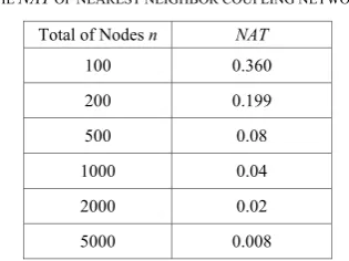
Total of Nodes n NAT

100 0.360 200 0.199 500 0.08 1000 0.04 2000 0.02 5000 0.008

and the averages are obtained. The results are shown in Table III (λ=0.8, <k>=10).

TABLE II.

THENAT OF NW SMALL-WORLD NETWORK

Total of Nodes n NAT

100 0.581 200 0.530 500 0.470 1000 0.429 2000 0.392 5000 0.362

Scale free network is a heterogeneity network which has power law degree distribution. BA model can build a scale free network dynamically based on characteristics of the growth and priority connection. Starting from a complete network with k +1 nodes, nodes will be added one by one. When a node is joined in the network, k/2

edges connecting this node and the existed nodes are also joined. Existed nodes with higher degree have a greater probability to be connected. Thus, we can build a scale-free network which has n nodes and the average degree is

k. NAT can be calculated according to the simulated BA network with different scales. To ensure the correctness of the results, each type of simulation experiments has conducted in 100 times and the averages are obtained. The results are shown in Table IV (λ=0.8, <k>=10).

TABLE III.

THENAT OF ER STOCHASTIC NETWORK

Total of Nodes n NAT

100 0.614 200 0.572 500 0.523 1000 0.489 2000 0.457 5000 0.419

TABLE IV.

THENAT OF BASCALE FREE NETWORK

Total of Nodes n NAT

100 0.623 200 0.585 500 0.546 1000 0.524 2000 0.500 5000 0.450

In nearest neighbor coupling network, each node has the same degree (k=10). The distances of node pairs are evenly distributed from 1 to n/k. When the total number of nodes n is increasing, there are many long distance

node pairs arisen. So NAT is reduced significantly following the increase of n. Although in NW network, there are only a few random edges, nodes can be linked with distant nodes by these random edges. Thus, distances of node pairs are shortened. So NAT in NW network is higher than in the nearest neighbor coupling network. And with the increase of n, NAT has slowly down. Like NW work, ER network also has the character of the small world. So, the total number of nodes has little effect on NAT. Because all edges are random in ER network, compared to NW network, the distances of nodes pairs are shorter in general. So with the same scale,

NAT in ER network is higher than in NW network. In BA network, the total number of nodes n also has little effect on NAT because of the character of the small world. There have a few nodes with a great degree in the BA network. Taking these nodes as intermediaries, nodes pairs in the BA network can contact by a short path. So, BA network has higher NAT. The data in the tables above have fully proved the characteristics of NAT in different complex networks.

B. Analysis of Network Node Average Trust

Definition 5: Network Node Average Trust (NNAT) is the arithmetic mean value of trusting values of nodes pairs including a certain node. NNAT of node i is calculated by the following formula.

∑

≠ =

−

= N

i j j

T

NNATi

1

1 1

The following formula is another method to calculate the NNATi. Counti(x) is equivalent to the total count of the nodes pairs which include node i and the distance is x.

∑

=

−

= 1

1

) ( 1

1 N

x

x x Counti N

NNATi

λ

The average trust of a node can reflect how degree this node trusts on others or be trusted on by others. The node i with high NNAT indicates that information or opinion from this node is easier to be accepted by others and the information appeared in the network may be sent to this node with a higher probability as soon as possible.

To analyze the power of different individuals influence on others in a complex network, NNAT of nodes in different types of complex are calculated. NAT is calculated with assuming λ = 0.8 and average degree <k> = 10.

TABLE V.

THENNAT OF NODES IN NEAREST NEIGHBOR COUPLING NETWORK

Total of Nodes n NNAT of Nodes

500 0.08 1000 0.04 2000 0.02

scale are shown in Table V which we can find the data are same as Table I.

Simulation according to NW model is used to build several small world networks. Then, we can calculate the

NNAT of nodes in these small-world networks. Obviously

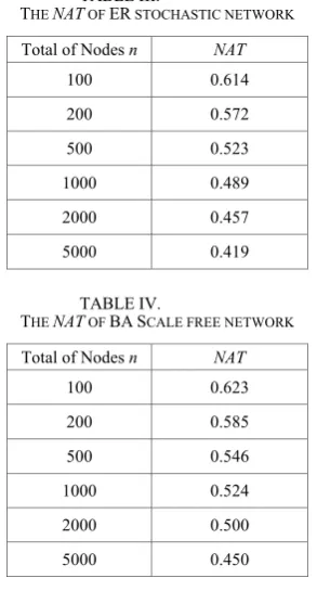
NNAT of a node depends on its degree. NNAT of nodes are calculated and classified according their degrees in NW networks with the total of nodes are 500, 1000 and 2000 (n=500, 1000, 2000). The result is shown in Figure 1 (a), (b) and (c). Here, x-axis is the node degree, y-axis is NNAT.

(a) n=500

(b) n=1000

(c) n=2000

Figure 1. NNAT of the nodes in NW networks

Nodes with high degrees also have high NNAT. The rule can be found from (a), (b) and (c) of Figure 1. Comparing (a), (b) and (c) of Figure 1, we can find that the total of nodes has an effect on the NNAT of nodes in the network, just as it effect on NAT of the network. With the same degree, nodes in the large scale network have less NNAT while nodes in the small scale network have

bigger NNAT. For example, assuming the node degree is 8, NNAT is about 0.45 in the network with n=500

(shown in (a) of Figure 1). In the network with n=1000, it is less than 0.41(shown in (b) of Figure 1). In the network with n=1000, it is about 0.37(shown in (c) of Figure 1). Comparing the data in Figure 1 with the data in Table V, we can find that the structure also has a certain effect on NNAT. In same condition, NNAT of a node in a small world network is high than NNAT of a node in a coupling network. For example, while n=1000, NNAT of nodes in nearest neighbor network is 0.04 (see it from the second row in Table V), whereas NNAT of nodes in NW network is more than 0.4 (see it from (b) of Figure 1).

(a) n=500

(b) n=1000

(c) n=2000

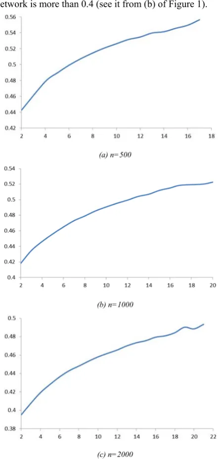
Figure 2. NNAT of the nodes in ER networks

The difference of NNAT in a small world network can also be calculated. When n=500, the difference between maximum and minimum of NNAT is about 0.09. When

different nodes in a small world network have a little difference of their NNAT.

Simulation according ER model is used to build several stochastic networks with the total of nodes are 500, 1000 and 2000 (n=500, 1000, 2000). Then, we can calculate the NNAT of nodes in these stochastic networks. The result is shown in Figure 2 (a), (b) and (c).

From (a), (b) and (c) of Figure 2, High degree nodes has high NNAT can be also found. And with the same degree, nodes in the large scale network have less NNAT

while nodes in the small scale network have bigger NNAT. These two characteristics of NNAT in stochastic networks are same as small world networks. Comparing Figure 1 with Figure 2, we can find that the structure of stochastic networks has more positive effect on NNAT than little word network. In same condition, NNAT of node in stochastic network is higher than NNAT of node in a small world network. For example, while n=1000,

degree=10, NNAT of nodes in NW network is about 0.43 (see it from (b) of Figure 1), while NNAT of nodes in ER network is about 0.49 (see it from (b) of Figure 2).

When n=500, the difference between maximum and minimum of NNAT is about 0.125. When n=1000, the difference is about 0.10. When n=2000, the difference is about 0.085. They are all more than that in a small world network. It indicates that different nodes in stochastic have some difference in their NNAT, but not very sharp.

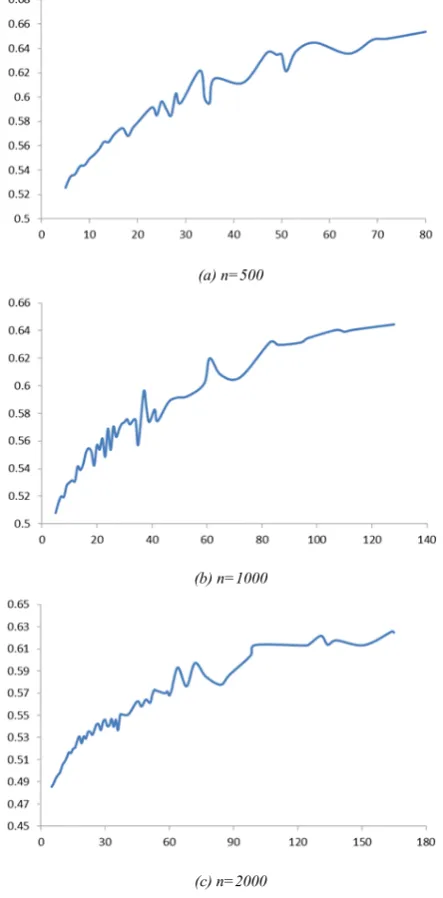
Simulation according BA model is used to build several scale free networks with the total of nodes are also 500, 1000 and 2000 (n=500, 1000, 2000). Then, we can calculate the NNAT of nodes in these scale free networks. The result is shown in Figure 3 (a), (b) and (c).

Characteristics of NNAT in small world networks and stochastic networks are also can find in scale free networks from (a), (b) and (c) of Figure 3. More, comparing Figure 3 with Figure 1 and Figure 2, we can find that the structure of scale free networks has most positive effect on NNAT. In same condition, NNAT of a node in a scale free network is highest. For example, while n=1000, degree=10, NNAT of nodes in a BA network is about 0.53 (see it from (b) of Figure 3).

When n=500, the difference between maximum and minimum of NNAT is about 0.13. When n=1000, the difference is about 0.14. When n=2000, the difference is about 0.15. They are all more than other types of networks. In a scale free network, there always have a few nodes with high NNAT whatever the total of nodes in the network is, because there have very high degree nodes in a scale free network. In coupling network, all nodes have the same degree. In small world network and stochastic network, the node degree is concentrated around the average degree of the network. So, the NNAT

of nodes have little difference, especially in the network with large scale. Comparing with Figure 1 and Figure 2, it is not as smooth as Figure 3, but the variation trends are same. Nodes with high degrees also have high NNAT.

In BA network with power law degree distribution, the degrees of nodes are dispersed. There have a few great degree nodes and many small degree nodes. The NNAT of the nodes with a great degree are high of course.

Interestingly, the NNAT of small degree nodes is also higher. In BA network, NNAT of different nodes with different degree have a little different. With the same degree, nodes in the BA network have higher average trust than nodes in the ER network. Even if the node has less degree, it can reach other nodes quickly by the intermediate nodes with a great degree.

(a) n=500

(b) n=1000

(c) n=2000

Figure 3. NNAT of the nodes in BA networks

C. Analysis of a Certain Instance

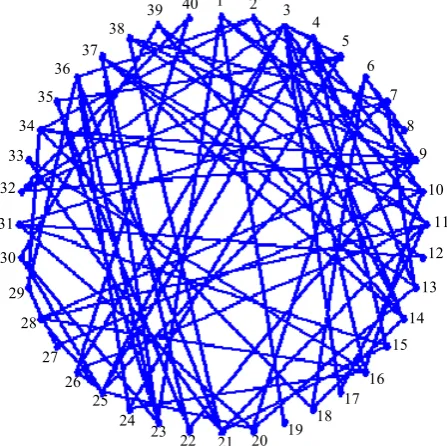
In this section, a miniature social network is shown in figure 4 as an example.

There are 40 nodes in this instance. It is a stochastic network. The average degree is 4. Calculating NNAT of every node, the result is shown in Table VI taking λ=0.8. Node 3 has the maximum value of NNAT. It is 0.6326. Node 19 has the minimum value of NNAT. It is 0.4651. NAT of this network can also be calculated. It is 0.5620.

know the message. The information will be disseminated all over the network even if only a node has known it at first. But different resource of the information has a different effect on information dissemination. Many papers have proved it [17-19]. Trust has an effect on information dissemination. Assuming the probability of information dissemination is 0.1 and taking Node 3 as the information resource, all will know the message after 38 rounds of dissemination in average. If Node 19 is the information resource, all will know the message after 49 rounds of dissemination in average. High NNAT is beneficial to an information resource.

Figure 4. a Miniature Social Network

TABLE VI.

NNAT OF NODES IN THE INSTANCE

i NNATi i NNATi i NNATi i NNATi 1 0.5763 11 0.5958 21 0.5896 31 0.5256 2 0.5671 12 0.5035 22 0.5571 32 0.5829 3 0.6323 13 0.5645 23 0.5896 33 0.5215 4 0.6021 14 0.5995 24 0.5433 34 0.5752 5 0.5678 15 0.5545 25 0.6109 35 0.5394 6 0.5671 16 0.5870 26 0.5611 36 0.5896 7 0.5599 17 0.5319 27 0.4870 37 0.5837 8 0.5071 18 0.5427 28 0.5980 38 0.5914 9 0.6228 19 0.4651 29 0.5256 39 0.5524 10 0.5837 20 0.5625 30 0.5630 40 0.4996

To investigate the effect a node on others, assuming opinions of Node 3 and Node 19 on something are at opposite poles (10 indicates strongest support while -10 indicates strongest support opposition), others will be effect by them in different ways and different extent according trusting values. The opinions of other nodes can be estimated by the following formula.

10 10 ,19 3

,× − ×

=

_T

_T

E

Here Ei is the estimated value indicating the opinion of the node i. The result is shown in Table VII.

TABLE VII.

OPINION ESTIMATED VALUE OF NODES IN THE INSTANCE

i Ei i Ei i Ei i Ei 1 -2.88 11 3.904 21 2.304 31 1.8432 2 2.304 12 1.024 22 0 32 2.88 3 10 13 2.304 23 -1.28 33 2.304 4 2.88 14 3.904 24 2.304 34 0 5 3.904 15 2.304 25 3.904 35 1.28 6 0 16 2.88 26 4.7232 36 0 7 2.304 17 4.7232 27 0 37 1.28 8 1.024 18 2.304 28 1.28 38 1.28

9 0 19 -10 29 0 39 2.304

10 0 20 2.304 30 1.28 40 2.304 Ei can be used to form a basic evaluation according opinion of others before he knew little. If the trust value

Tij is high, they will effect on each other more. In Table VII, if Ei>0, it indicates that the node i is more close to Node 3. While Ei<0 indicates that the node i is more close to Node 19. The average of Ei is 1.7152, more than 0. It is because NNAT of Node 3 is higher than NNAT of Node 19. In many case, especially in online shopping and estimate, trust s very important, we can see it in many papers [20-24]. NNAT provides a new way in this area.

IV. CONCLUSION

Trusting value can measure close degree between two individuals in the social network. Network Node Average Trust can measure the general influences of members in the network. Network Node Average Trust can measure the influence of an individual on others. NAT and NNAT

of network are impacted by network topology. The network with characteristics of the small world and the free scale has high NAT. More scattering degree distributes, the higher NAT is. For networks with the same size and average degree, the sequence according to

NAT increasing is coupled network, the small-world network, random network and scale free network. NNAT

is an increasing function of the node degree. It is also affected by the network topology like NAT. Nodes in the scale free network have high NNAT than others under the same condition. So, we can draw the conclusion that the scale free network is most conducive to the information transmission and communication.

Many methods based on mathematical statistics are also used to research dissemination rules in the social network. Comparing these methods, trusting relation provides a static datum to analyze and estimate the situation of information dissemination in a certain network only according the network itself. Trusting values between individuals with direct contacts are the primitive input datum. They are one of the key factors to determine how far the information can be disseminating and how many people will receive it. The other key factor

1 2 ₃ 4

5 6

7 8

9

10 11 12 13 14 15 16 17 18 19 20 21 32

33

22 23 24 25 26 27 28 29 30 31

34 35

36 37

is the structure of the social network. Further, trusting relation can also be used in some other social activities. Whether persons can communicate well or not is determined by their trusting value. What degree a person’s opinion will be accepted by others is determined by its NNAT. The collaboration of the network is determined by NAT of the social network. The research of trusting relationship in complex network provides a universal way to analyze and resolve the social activities from the view of both the individual and the whole.

REFERENCES

[1] Wu Peng, “Social Network Analysis Layout Algorithm under Ontology Model”, Journal of Software, vol. 6, pp. 1321-1328, July 2011.

[2] Yu-Feng Chou, Hsin-Heng Huang, and Ray-Guang Cheng, “Modeling Information Dissemination in Generalized Social Networks”, IEEE Communications Letters, vol. 17, pp. 1356-1359, July 2013.

[3] He Xiaolan, “Prediction Model of Network Information Dissemination”, Journal of Networks, vol. 8, pp. 1112-1120, May 2013.

[4] Anagnostopoulos C. , Hadjiefthymiades S. and Zervas E. , “An analytical model for multi-epidemic information dissemination”, Journal of Parallel and Distributed Computing, vol. 71, pp. 87-104, January 2011.

[5] Hui Chen, “Relationship between Motivation and Behavior of SNS User”, Journal of Software, vol. 7, pp. 1265-1272, Jane 2012.

[6] Shijun Li, “Belief Reasoning Recommendation Mashing up Web Information Fusion and FOAF”, Journal of Compters, vol. 5, pp. 1885-1892, December 2010.

[7] Mohammad M. R. Chowdhury, Sarfraz Alam and Zahid Iqbal, “Sociality brings Security in Content Sharing”,

Journal of Parallel and Distributed Computing, vol. 5, pp. 1839-1845, December 2010.

[8] Thomas H. Cormen，_{Charles E. Leiserson}，_{Ronald L.}

Rivest and Clifford Stein, Introduction to Algorithms, Beijing: China Machine Press, 2006, pp. 452-524.

[9] Mark Allen Weiss, Data Structures and Algorithm Analysis，_{Beijing: Post & Telecom Press, 2007, pp.}

123-202.

[10]Anany Levitin, Introduction to the Design and Analysis of Algorithms, 2rd _{ed., Beijing: Tsinghua University Press,} 2007, pp. 312-376.

[11]Kyle Loudon, Mastering Algorithms with C, Beijing: China Machine Press, 2012, pp. 174-235.

[12]M. H. Alsuwaiyel, Algorithms Design Techniques and Analysis, Beijing: Publishing House of Electronics Industry, 2010, pp. 23-89.

[13]Guo ShiZhe and Lu Zheming, Complex Network Basic Theory, Beijing: Science Press, 2012, pp. 143-146.

[14]He Daren and Liu Zonghua, Complex Systems and Complex Networks, Beijing: Higher Education Press, 2009, pp. 17-58.

[15]Liu Ying, Study on Knowledge Communication from Complex Network Perspective, Beijing: China Renmin University Press, 2012, pp. 12-89.

[16]Wang Xiaofan, Li Xiang and Chen Guanrong, Complex Network Theory and Application, Beijing: Tsinghua University Press, 2006, pp.126-164.

[17]Weihui Dai, “Emergency Event: Internet Spread, Psychological Impacts and Emergency Management”,

Journal of Computers, vol. 6, pp. 1748-1755, August 2011. [18]Dong Cheng, “Is Value Sufficient? Empirical Research on the Impact of Value and Trust on Intention”, Journal of Software, vol. 6, pp. 124-131, January 2011.

[19]Bo Xhang and Yang Xiang, “Trust-aware Information Dissemination in Social Network”, Applied Mechanics and Materials, vol. 121-126, pp. 2400-2404, July 2012. [20]Chen Hui, “Personality's Influence on the Relationship

between Online Word-of-mouth and Consumers' Trust in Shopping Website”, Journal of Software, vol. 6, pp. 265-272, February 2011.

[21]Bailing Liu, “Efficient Trust Negotiation based on Trust Evaluations and Adaptive Policies”, Journal of Computers, vol. 6, pp. 240-245, February 2011.

[22]Chien-Chung Tu, “Perceived Ease of Use, Trust, and Satisfaction as Determinants of Loyalty in e-Auction Marketplace”, Journal of Computers, vol. 7, pp. 645-652, March 2012.

[23]Dongyan Jia, Fuzhi Zhang and Sai Liu, “A Robust Collaborative Filtering Recommendation Algorithm Based on Multidimensional Trust Model”, Journal of Software,

vol. 8, pp. 11-18, January 2013.

[24]Hui Chen, “The Influence of Perceived Value and Trust on Online Buying Intention”, Journal of Software, vol. 7, pp. 1655-1622, July 2011.

Juan Li was born in Jiangsu Province, China in 1977. She