ISSN: 2278-067X, Volume 1, Issue 10 (June 2012), PP.23-28
www.ijerd.com
Minimum Spanning Tree in Fuzzy Weighted Rough Graph
S. P. Mohanty
1, S. Biswal
2, G. Pradhan
3 1,2,3Department of Mathematics, College of Engineering and Technology, Techno Campus, Ghatikia, Bhubaneswar-751003, India
Abstract––The minimum spanning tree of a connected graph has many applications in different field of knowledge. In many real world problems the input data are often imprecise due to incomplete or non-obtainable information. This paper is intended to find minimum spanning tree on a rough graph where the edges have fuzzy weights. The Boruvka algorithm has been used to find the minimum spanning tree and signed distance ranking method has been used for ranking fuzzy numbers. Triangular fuzzy numbers are used as the weight of the edges.
Keywords and Phrases––Triangular fuzzy number, Ranking of fuzzy numbers, Rough set, Rough graph, Boruvka algorithm.
I.
INTRODUCTION
Many optimization problems can be tackled using graph theory. The classical graph theory may not be useful to deal with the problems where the data related to the graph such as weights attached to the vertices or edges, nature of connectivity between the vertices are imprecise. The fuzzy set theory can be effectively used to deal with these types of problems. But due to lack of proper information regarding the nature of connectivity between the vertices, the fuzzy set theory is also failed to handle the problems. T. He et al [5][6][7] have developed rough graph where they have applied rough set theory to attributed graphs. An attribute set was first assigned to edges of a graph. Given a subset R of the attribute set, there is associated an equivalences relation, based in which R-rough graph is defined. If the vertices of a graph are connected through edges denoting different possible relationships, it is required to quantify some attributes as the strength of relationship. The strength of relation can be deterministic where we can use crisp number, if the strength of relationship is imprecise, we can use fuzzy number.
This paper is intended to find the minimum spanning tree on a rough graph as developed by T.He et al, where the edges have fuzzy weights. The Boruvka algorithm has been used to find the minimum spanning tree and signed distance ranking method as suggested by J.S. Yao and F.T Lin [1] has been used to rank two fuzzy numbers. We have also used fuzzy triangular number as the weight of the edges.
This paper is organized as follows: some prerequisite related to fuzzy numbers, signed distance ranking methods are given in section-II. Various definitions related to rough graph are given in section III and section IV presents different algorithms to find the lower and upper approximations of rough graph and the minimum spanning tree of a fuzzy weighted rough graph. We have given one numerical example in section V to implement the algorithm. Finally in section VI, we conclude the paper with a suggestion for further work.
II.
FUZZY NUMBER AND SIGNED DISTANCE RANKING
A. Fuzzy number
All definitions and discussion are based on the definition of fuzzy set, fuzzy numbers. For the sake of completeness of the work, we introduce here the following definitions related to our work.
1) Definition : The level λ triangular fuzzy number
A
,0< λ ≤ 1 , denoted by
A
= (a, b, c ; λ ) is a fuzzy set defined on R with the membership function defined as
(
x
)
A
= λ (x – a)/ (b –a), a ≤ x ≤ b = λ (c – x) /(c – b), b ≤ x ≤ c = 0 otherwiseThe family of all level λ fuzzy numbers be denoted by FN (λ) = { (a, b, c ; λ)| a, b, c є R and a < b < c }
In addition, for λ = 1 , (a, b, c ; λ ) is a triangular fuzzy number and denoted by (a, b, c).
2) Definition: A fuzzy set
A
defined on R is called an interval–valued fuzzy set having the following membership function
A
= { (x ,[
AL(
x
),
AU(
x
)]
)} where x є R , 0 ≤
AL(
x
)
AU(
x
)
1
.Symbolically,
A
is denoted by [
A
L
,
A
U] for all x є R . The membership grade of x in
A
lies in the interval
)]
(
),
(
[
ALx
AUx
. In particular ifA
L = ( a, b, c ; λ ) and
A
U = ( p, b ,q ; ρ ) where 0 < λ ≤ ρ ≤ 1 , p < a < b< c <q, we get
A
= [ a, b, c ; λ ) , ( p, b, q ; ρ )] which is called the level ( λ , ρ ) interval–valued fuzzy number . Then themembership function of
A
)
(
x
LA
= λ (x - a) / (b - a), a ≤ x ≤ b = λ(c - x ) / (c - b) , b ≤ x ≤ c = 0 otherwise)
(
x
UA
= ρ (x - b) / (b - p), p ≤ x ≤ b = ρ(q - x ) / (q - b), b ≤ x ≤ q = 0 otherwiseThe family of all (λ , ρ ) interval–valued fuzzy numbers be denoted by FN ( λ , ρ)
3) Definition: Let
A
= ( a, b, c, λ ) and
B
= ( p, q, r, λ ). We have ,
)
,
,
,
(
a
p
b
q
c
r
B
A
4) Definition : Let
A
= [
A
L
,
A
U
] = [( a1, b1, c1, λ ) ,(p1 ,b1 ,q1 , ρ)] and
B
= [B
L
,
B
U
] = [(a2 ,b2, c2 , λ)
,(p2, b2, q2, ρ) ] be two interval- valued fuzzy numbers , then the binary operation
is defined byA
B
=]
,
[
A
L
B
LA
U
B
Uwhere,
A
L
B
L
(
a
1
a
2,
b
1
b
2,
c
1
c
2;
)
and
A
U
B
U
(
p
1
p
2,
b
1
b
2,
q
1
q
2;
)
B. Signed distance ranking of fuzzy numbers:
5) Definition: For b,0 є R , the signed distance of b measured from 0 is defined by
d
*( b ,0 ) = b . For any closed interval[a, b] , the signed distance of [a, b] measured from 0 is defined by
d
*([a, b],0) = (a + b)/2. For any two disjoint closed intervals [a, b] and [c, d] , the signed distance of [a, b] U [c, d] measured from 0 is defined by
d
*( [a, b] U[c, d] ,0) = [d
*([a, b],0) +d
*([c, d],0) ] / 2For
A
= [(a, b, c; λ) ,(p, b, q; ρ)] FN(λ, p) , 0 < λ < ρ ≤ 1, the signed distanced of
A
measured from
0
is defined by
*
d
(A
,
0
) =1/8 (6b + a + c + 4p + 4q) + 3λ/ρ (2b – p - q)
For
A
=[(a1,b1,c1; λ),(p1,b1,q1; ρ)] and
B
= [(a2,b2,c2; λ), (p2,b2,q2; ρ)] *
d
(A
B
),0
) =
d
*(A
,0
) +
d
*(B
,
0
)6) Definition: For
A
=[(a1, b1, c1; λ),(p1, b1, q1; ρ)] and
B
=[(a2, b2, c2; λ),(p2, b2, q2; ρ)] , 0 < λ < ρ ≤ 1, the ranking of
interval-valued fuzzy numbers on FN(λ, ρ) are defined by
A
<B
iff
d
*(A
,
0
) <
d
*(B
,
0
)
A
≈B
iff
d
*(A
,
0
) =
d
*(B
,
0
)
7) Definition: For 0 < λ ≤ 1 ,
A
= (a, b, c, λ) FN(λ) the signed distance of
A
measured from
0
is defined by d (
A
,
0
) = ¼ ( 2b + a +c).For ,
A
= (a, b, c, λ) and
B
= ( p, q, r ,λ) є FN(λ),
d(
A
B
),0
) =d (
A
,
0
) + d (
B
,
0
).
8) Definition: For ,
A
= (a, b, c, λ) and
B
= ( p, q, r ,λ) FN(λ), 0 < λ ≤ 1 , the ranking of level λ fuzzy number on
FN(λ) are defined by
A
<B
iff
d
(
A
,0
) <
d
(
B
,0
)
A
≈B
iff
d
A
(
,0
) =
d
(
B
,0
)
III.
WEIGHTED ROUGH GRAPH
In this section all definitions and discussions are based on the work of T. He et al [5] . For the sake of completeness we introduce here.
A. Rough graph.
9) Definition : Let U = (V, E ) be the universal graph where V = {v1,v2,…...vn} is the set of vertices and E= U ek(vi,vj) is
the edge set on U , where the edge ek is endued with vertex attribute (vi,vj). Let R = { r1,r2………….r|R|} be the attribute set
on U. For any attributes set R
R on E, the elements of E can be divided into different equivalence classes R(e). For any graph T = (W,X) , where W
V and X
E , the graph is called R-definable graph or R-exact graph if X is the sum of equivalence classes. Conversely, graph T is called R- undefinable graph or R- rough graph. For R-rough graph , two exact graphs R (T) = (W, R(X)) andR (T) = (W,R(X)) can be used to define it approximately, whereR (X) = { e E | R(e) X ≠ф }
The graph R(T) and R(T) are called R-Lower and R-upper approximation graph of T .The pair of graph ( R(T) ,R(T)) is called R- rough graph. The set bnR(X) = R (X) - R (X) is called the R–boundary of edge set X of T.
Property 1: The graph T = (R(T) ,R (T)) is exact iff R(X(T))=R(X(T)) and is a rough graph iff R(X(T)) ≠R(X(T)).
Property 2 : The rough graph T = (R(T) ,R(T)) is a classical graph iff all the edges of T belong to the same edge equivalence class with respect to R.
B. The class connection of rough graph
10) Definition : A (vo,vn) surely class walk in rough graph T = ( R(T) ,R(T)) is a finite non – null sequence w =
n v v n v
v v
v
v
R
e
v
v
R
e
v
e
R
v
n n
]
[
.
.
...
]
[
]
[
1 2
1 1
0 1 2 1
0 , whose terms are alternatively vertex and edge equivalence class in
R(T). The surely class walk is called surely class path if vi ≠ vj for all i ≠ j where i, j = 0,1,2,3,….,n-1 .
Similarly, possibly class walk or class path can be defined analogously if the edge equivalence class are taken from R(T). 11) Definition :Two vertices u,v are called surely or possibly class connected if there is a (u,v) surely or possibly class path in R (T) orR (T) respectively.
12) Definition: A (vo,vn) surely class path or possibly class path is called a surely class cycle or possibly class cycle if vo =
vn.
13) Definition : A rough graph is called surely class tree, if it is surely class connected and does not contain surely class cycle. Similarly, a rough graph is called possibly class tree, if it is possibly class connected and does not contain possi bly class cycle.
14) Definition: For any rough graph T = (R(T) ,R(T)) , the surely class tree or possibly class tree H T is called surely or possibly class spanning tree if w(T) = w(H), where w(T) is the vertices set of T and w(H) is the vertices set of H
C. Fuzzy weighted rough graph
15) Definition : For the universe graph U = ( V,E), for all e E, we define the mapping w: e w(e) where w(e) is a fuzzy triangular number called the edge weight of e .
w(R(euv)) = f(w(e)) is called the class weight of edge equivalence class R(euv) , where e R(euv) and f is some function. In
our work f is taken as sum of all fuzzy weights of the elements of edge equivalence class.
Rough graph with the class weight of their edge equivalence class is called weighted rough graph. The weighted rough graph with fuzzy weights of the edges is called fuzzy weighted rough graph. In fuzzy weighted rough graph, the surely or possibly class spanning tree with the lightest class weight sum is called the surely or possibly class minimum spanning tree.
In this paper we have used signed distance ranking method to rank fuzzy weights and the minimum rank is considered to be the lightest weight in order to find the surely or possibly class minimum spanning tree .
IV.
ALGORITHMS
In this section , we give some algorithms to classify the edge sets as edge equivalence classes, lower and upper approximate graph of rough graph and using lower and upper approximate graph, we find the surely or possibly class minimum spanning tree.
let R ={ v1,v2,………….,vn} be the finite attribute set on U =(V,E) , the universe graph. For any attribute set R R
on E, E/R is the set of all equivalence classes which makes a partition of E. Two elements ei, ej E where i ≠ j are called in
the same kind if R(ei) = R(ej).
A. In this section we present the algorithm which gives the classification method to find the edges set of universe graph. In the algorithm three indexes are used : the index i points to the recent input object ei , the index s records the
classes E1 ,E2 …………..,Es which has been found, and the index j is one of the 1,2,…..s which is used to check whether
the recent input object ei satisfies Ej = R (ei) or not . Algorithm partition :
Step 1 : i=1 ,j=1, s=1 , E1 = { e1 }
Step 2 : if i = | E |, then complete the classification and we have E/R = { E1, E2, ...., Es } else
go to step 3 Step 3 : i = i+1 ,j =1
Step 4 : if j = s , then establish a new class
Step 5 : s = s+1 , Es = { ei } and go to step 2 to input the next object
Step 6 : if j < s go to step 7 . Step 7 : j = j+1 , go to step 8.
Step 8 : if Ej = R (ei) then ei Ej , go to step 2 else go to step 4 to check the next Ej .
to E/R by using the following algorithm lower and algorithm upper respectively so that we can get the lower approximate graph R(T) and the upper approximate graphR (T ). Given the universe graph U = ( V,E ) , let E/R = {E1 , E2 ,………, Es}
,1≤ s ≤ |E|
Algorithm lower : Step 1 : j =1 , L =ф .
Step 2 : if Ej X , then L = L Ej .
Step 3 : if j = s ,then stop and we have R(X) = L else go to step 4 to check next Ej
Step 4 : j = j+1 and go to step 2 .
Algorithm upper : Step 1 : j = 1 , R = ф,
Step 2 : if Ej X ≠ ф , then R = R Ej
Step 3 : if j = s , then stop and we have R (X ) = R else go to step 4 to check next Ej
Step 4 : j= j+1 and go to step 2.
C. In this section we describe Boruvka’s algorithm to find the minimum spanning tree(MST). It is considered as a greedy algorithm like Kruskal’s algorithm. However, unlike Kruskal’s algorithm, which merges two components in a step, in a single step of Boruvka’s algorithm every component is involved in a merger. The basic idea in this algorithm is to contract simultaneously the lightest edges incident to each of the vertices in the graph. For a graph G, we take a forest F initially with all the vertices of G. The algorithm continually adds edges to the forest F and contract G( and simultaneously F) across any of the edges already in F. At the end of the algorithm, F and G are eventually reduced to a single vertex. We must keep a separate list of all edges added to F. When the algorithm ends, the MST is specified by this list. In a contraction, only the lightest edge needs to be retained out of any number of multiple edges.. The process of contracting the lightest edge for each vertex in the graph is called Boruvka step.
The implementation of Boruvka step is the following: 1. Mark the edges to be contracted
2. Determine the connected components formed by the marked edges 3. Replace each connected component by a single vertex
4. Eliminate the self loops and multiple edges created by these contraction
5. If G’ be the graph obtained from G after a Boruvka step. The MST of G is the union of the edges marked for contraction during this step with the edges in the MST of G’
Algorithm Boruvka step:
For any graph G = (V , E), let Gi = (Vi , Ei) where Vi
V and Ei
ELet F be the forest of MST edges and G’ be the contracted graph. Step 1: F = φ
Step 2: for all euv Ei do
if w(euv) < u. minWeight then
u.minWeight = w(euv)
u.minEdge = euv
end if
Step 3: for all euv Ei do
if w(euv) < v. minWeight then
v.minWeight = w(euv)
v.minEdge = euv
end if Step 4: for all v ε V do
put v.minEdge in F end for
Step 5: Gi = contract (Gi)
Step 6: F = contract (F)
The graph remaining after the ith iteration is the input to the ( i+1)st iteration . The iteration continues till the graph left with one vertex on which case the algorithm halts. The output spanning tree is the union of the set of lightest edges selected taken over all iterations. In the implementation of the above algorithm, we need to store fields min Edge and min Edge weight for each vertex.
In our case, as the weights of edges are supposed to be fuzzy triangular numbers, the edge having lower rank between two fuzzy triangular number is considered to be the light weight edge in comparison to the others. We have used signed distance ranking method as discussed in section 2 to rank two triangular fuzzy numbers .
D. Combing the above four algorithms, we give the algorithm MST for exploring the minimum spanning tree in weighted rough graph.
Algorithm MST :
Step 1 : Input a knowledge system (U, R) where U = (V,E ) , R = { r1,r2………….rn} , R R of the rough graph T =(
W,X).
Step 3 : Apply algorithm lower and algorithm upper to X respectively to get the lower approximate R(X) and the upper approximate R (X) of X .
step 4 : For the lower approximate graph R (T) = (W, R (X)) of R (T) is still class connected for some edge equivalence class Ei , apply algorithm Boruvka step to R (T)
corresponding to every Ei , get the surely class spanning tree.
Step 5 : If R (T) is not class connected for all edge equivalence class Ej ,j =1,2,……..s then there
is no surely class minimum spanning tree .
Step 6 : Apply algorithm Boruvka step to the upper approximate graph R (T) = (W, R (X)) corresponding to all Ej ,j =1,2,……..s to get the possibly class minimum spanning tree.
V.
NUMERICAL EXAMPLE
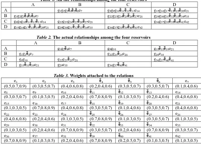
In this section, we give one numerical example to implement the algorithm discussed. Let there are four water reservoirs A, B, C, D in a city where water is drawn from three rivers and also drawn from the ground. We have defined three kinds of relations such as, two reservoirs are related if they draw water either from the same river or from different rivers or from the ground which are denoted by ei, ēj, ek respectively. As there are three rivers each relation of first and
second kind have three types of relations. With the existing knowledge, we can only know about how many sub-relations exist in every kind, but we cannot distinguish the sub-sub-relationships of the same kind. The purpose is to find the extremely conflicting relation (water is drawn from different rivers) among them. The weight corresponding to each relation is given in form of triangular fuzzy number which denotes the degree of weakness of the relation to make use of our algorithm. The class weight is considered as the sum of the edge weights and comparing the class weights, we use the signed distance ranking method as discussed in previous section. The edge having lesser rank is considered to have less weight.
Table 1. All the relationships among the four reservoirs
A B C D
A e1e2e3ē4ē5ē6e7 e8e9e10ē11ē12ē13e14 e15e16e17ē18ē19ē20e21
B e1e2e3ē4ē5ē6e7 e22e23e24ē25ē26ē27e28 e29e30e31ē32ē33ē34e35
C e8e9e10ē11ē12ē13e14 e22e23e24ē25ē26ē27e28 e36e37e38ē39ē40ē41e42
D e15e16e17ē18ē19ē20e21 e29e30e31ē32ē33ē34e35 e36e37e38ē39ē40ē41e42
Table 2. The actual relationships among the four reservoirs
A B C D
A e1e2ē4e7 e9e10 e15ē18ē19e21
B e1e2ē4e7 e22e23ē25e28 e29e35
C e9e10 e22e23ē25e28 e36e37ē40ē41
D e15ē18ē19e21 e29e35 e36e37ē40ē41
Table 3. Weights attached to the relations
e1 e2 e3 ē4 ē5 ē6 e7
(0.5,0.7,0.9) (0.3,0.5,0.7) (0.4,0.6,0.8) (0.2,0.4,0.6) (0.3,0.5,0.7) (0.3,0.5,0.7) (0.1,0.4,0.6)
e8 e9 e10 ē11 ē12 ē13 e14
(0.3,0.5,0.7) (0.1,0.3,0.5) (0.2,0.4,0.6) (0.7,0.8,0.9) (0.1,0.3,0.5) (0.2,0.4,0.6) (0.4,0.6,0.8)
e15 e16 e17 ē18 ē19 ē20 e21
(0.1,0.3,0.5) (0.7,0.8,0.9) (0.4,0.6,0.8) (0.3,0.5,0.7) (0.1,0.4,0.6) (0.3,0.5,0.7) (0.4,0.6,0.8)
e22 e23 e24 ē25 ē26 ē27 e28
(0.4,0.6,0.8) (0.2,0.4,0.6) (0.1,0.3,0.5) (0.7,0.8,0.9) (0.1,0.3,0.5) (0.3,0.5,0.7) (0.1,0.3,0.5)
e29 e30 e31 ē32 ē33 ē34 e35
(0.1,0.3,0.5) (0.2,0.4,0.6) (0.7,0.8,0.9) (0.3,0.5,0.7) (0.2,0.4,0.6) (0.7,0.8,0.9) (0.3,0.5,0.7)
e36 e37 e38 ē39 ē40 ē41 e42
(0.7,0.8,0.9) (0.1,0.3,0.5) (0.2,0.4,0.6) (0.7,0.8,0.9) (0.2,0.5,0.7) (0.1,0.3,0.5) (0.1,0.3,0.5)
Taking A, B, C, D as vertices and e1 to e42 as edges, we can get the universe graph U. A rough graph X can be
U = { ē4 ,ē5 ,ē6, ē11 ,ē12 ,ē13, ē18, ē19 ,ē20, ē25 ,ē26 ,ē27, ē32 ,ē33 ,ē34, ē39 ,ē40 ,ē41}
X = { ē4, ē18, ē19, ē25, ē40, ē41 }
)
(
X
R
{ ē4 ,ē5 ,ē6, ē18, ē19, ē20,ē25, ē26, ē27, ē39, ē40,ē41}A
ē4 ,ē5 ,ē6 ē18, ē19, ē20
B D
ē39 ,ē40 ,ē41
C
Fig.1 Possibly conflicting MST
VI.
CONCLUSION
In this paper we have considered the weight of each edge as fuzzy triangular number . The weight can be considered as fuzzy trapezoidal number or interval – valued fuzzy number depending on the nature of the problem and impreciseness. Out of several ranking methods between fuzzy numbers we have considered the signed distance ranking method. Other methods can be used in ranking of fuzzy numbers. This paper intends the application field of rough graph with imprecise of the data.
Further, we have used Boruvka algorithm for finding minimum spanning tree as this method is more suitable for parallel implementation which can be further investigated for rough graph .
REFERENCES
[1]. Jing-Shing Yao and Feng-Tse Lin, “ Fuzzy shortest path network problems with uncertain edge weight”, Journal of Information Science and Engineering, Vol-19, pp 329-351, 2003
[2]. M. Liang, B. Liang, L. Wei, X. Xu, “Edge rough graph and its application”, Proc. Of eighth International Conference on Fuzzy Systems and Knowledge Discovery, pp 335-338, 2011
[3]. R. L. Graham and P. Hall, “On the history of the minimum spanning tree problem”, Annals of the History of Computing, Vol-7 No.1, pp 43-57, 1985
[4]. Sun Chung and Anne Condon,” Parallel implementation of Boruvka’s minimum spanning tree algorithm”, Technical report 1297, Computer Science Department, University of Wisconsin, Madison, 1996
[5]. T. He, Y. Chan and K. Shi, ”Weighted rough graph and its application”, Proceedings of sixth IEEE international conference on intelligent system design and application(ISDA 2006), Vol-1, IEEE Computer society, pp 486-491, 2006
[6]. T. He and K. Shi, “ Rough graph and its structure”, Journal of Shandong University, Vol-6, pp 88-92, 2006 [7]. T. He, P. Xue and K. Shi, “ Application of rough graph in relationship mining”, Journal of System
Engineering and Electronics, Vol-19, No. 4, pp 742-747, 2008