Seismic Displacement Evaluation Chart Method for Caisson Quay Walls Improved by the Vibro-Compaction Method

http://www.sciencepublishinggroup.com/j/es doi: 10.11648/j.es.20180302.11

ISSN: 2578-9260 (Print); ISSN: 2578-9279 (Online)

Seismic Displacement Evaluation Chart Method for

Caisson Quay Walls Improved by the Vibro-Compaction

Method

Bin Tong

1

, Vernon Schaefer

2

, Yingjun Liu

3

1_{China Institute of Geo-environment Monitoring, Beijing, China} 2

Department of Civil, Construction and Environmental Engineering, Iowa State University, Ames, USA 3

China Ordnance Industry Survey and Geotechnical Institute, Beijing, China

Email address:

To cite this article:

Bin Tong, Vernon Schaefer, Yingjun Liu. Seismic Displacement Evaluation Chart Method for Caisson Quay Walls Improved by the Vibro-Compaction Method. Engineering Science. Vol. 3, No. 2, 2018, pp. 11-25. doi: 10.11648/j.es.20180302.11

Received: August 4, 2018; Accepted: August 21, 2018; Published: December 21, 2018

Abstract:

Gravity type caisson walls are a type of popular but easily damaged waterfront construction structure, especially in seismic regions. Various forms of mitigation measures have been successfully and economically applied to improve their performances under the influence of soil liquefaction. Establishment of an effective, reliable, and easily-implemented liquefaction remedial design process based on a commonly used ground improvement technology is important for routine practice. To solve this problem, the vibro-compaction method, as one the most widely used accepted liquefaction remediation method, is applied as the countermeasure to improve a gravity type quay wall damaged by seismic-liquefaction in this study. More than three hundred cases of numerical analyses with variations of the improved zone configurations, improved soil properties and levels of seismic excitation loading were conducted. Based on the results of the parametric study, numerous correlations among various improved zone configurations, improved relative densities of the soils, excitation level, and improved performances of the caisson-wall structure are established. Therefore, a simple chart design procedure based on the established correlations is proposed to estimate the improved residual displacement of gravity caisson quay walls remediated by the vibro-compaction method. The results can be used as a convenient reference for liquefaction mitigation of gravity caisson wall using vibro-compaction method in routine practice.

Keywords:

Gravity Caisson Quay Wall, Liquefaction Mitigation, Vibro-Compaction, Design Chart Method

1. Introduction

Gravity type quay walls, as a type of widely used port structures, could suffer severe deformation failure in earthquake events when the adjacent in-situ soil (foundation soil and backfill soil) are prone to liquefaction. Liquefaction remediation of such structures has drawn significant efforts over the last three decades after the Kobe earthquake in 1995.

Specially, by using the numerical or experimental methods, predicting the improved residual deformation of quay walls by considering the influence of in-situ soil liquefaction is a critical but difficult step in the routine remedial design program for caisson quay wall structures due to the restriction on time and cost efficiency. A highly sophisticated calculation is practically difficult for a routine

remediation project. Therefore, it is desirable to establish a simple estimation technique such as chart method for improved seismic deformation of quay walls.

The applicability of the effective stress analysis for improved seismic performance evaluation of gravity type quay wall was verified with the case history of a damaged quay wall in Rooko port during the 1995 Kobe earthquake [1]. However, the influences of various improvement features such as improved zone configurations and improvement extent on seismic deformation of caisson quay wall are rarely discussed.

extent (densification or cementation) and the volume of soil that is treated. The proposed chart-method can be used to predict the unimproved seismic deformation of gravity quay wall based on the wall height and width, thickness of foundation soil and backfill, the liquefaction resistance of backfill and foundation soil.

To overcome this problem, an improved seismic displacement evaluation chart method is proposed based on a comprehensive parametric studies using finite difference method FLAC 3D [2]. In this study, a comprehensive parametric study is conducted, by varying improvement parameters for a gravity quay wall subjected to various levels of seismic excitations, to establish a simple estimation technique for improved seismic deformation of caisson type quay walls. The primary objective of this paper is to develop such a simplified procedure for evaluating the order-of-magnitude improved displacement for a gravity quay wall.

2. Numerical Modeling Verification

The verification process in this study is divided into three major steps within a framework of a well-calibrated case history, which was damaged gravity type caisson quay wall in Kobe earthquake in 1995 [3, 4]:

(1)Unimproved benchmark: a detailed numerical simulation is conducted on a well-documented case history (damaged gravity type caisson wall) using a three dimensional finite difference FLAC3D [2]. (2)Remediation: after verification of the numerical

simulation, the vibro-compaction programs of different improvement design parameters were hypothetically applied to caisson-wall soil structure, and the improved performances achieved by different improvement scenarios were calculated.

(3)The correlations among improved deformations of the wall, improvement design parameters, and soil properties are established for improved seismic performance evaluation chart method.

The case history simulation, which is used as the unimproved framework, is verified based on two criteria: (1) the simulated caisson wall-soil system deformation pattern is compared to field observations [3]; (2) the calculated maximum EPWP is compared to the results measured from experimental testing based on [3, 4].

2.1. Soil Constitutive Model Verification

The numerical method used in this study utilizes the finite difference formulation of FLAC3D [2]. In the FLAC software, the Finn-model, is one of the “built-in” models to predict the nonlinear dynamic response with considering dynamic EPWP generation. The Finn model was developed by incorporating the empirical estimation of volumetric strain into the standard Mohr-Coulomb plasticity model [5, 6]. The Finn-model can capture the basic mechanisms that lead to liquefaction in sand or granular material. In the Finn-model, as mathematically presented in Equations 1 to 5, the volume change that leads to dynamic pore pressure build-up in sand

is a function of the material-dependent parameters C1, C2, C3

and C4, which can be determined based on relative density

(Dr%) and SPT blow count SPT (N1)60 of the soil being

simulated. The detailed description and the parameters determination procedure of Finn-model and the working mechanism of FLAC3D software can be found in [5, 6, 7, 8] or FLAC3D User’s Manual [2], and are not expanded herein. The Finn model is utilized to describe the soil stress-strain response and dynamic EPWP generation at small strain range or when EPWP ratio is less than 0.6. Equations 1 to 5 describe the Finn-model mathematically:

∆ = − + × (1)

∆ = exp − × (2)

= . (3)

= 7600 × 15 × % _&.' ( .' ₍₄₎

= 8.7 × % &( . ' (5)

C1, C2, C3, and C4 are material-specific fitting parameters

and primarily depend on relative density of the soil; ∆ is plastic volumetric strain change; is shear strain; (N1)60 the

corrected Standard penetration resistance blow count-SPT. C1

mainly controls the amount of volume strain increment and C2 mainly controls the shape of volumetric strain curve, and

both parameters can be obtained from simple shear tests for particular granular materials [9]. The key elastic and plastic parameters can be expressed in terms of relative density, Dr or normalized Standard penetration test blow count values.

The Finn-model is utilized to describe the soil stress-strain response and dynamic EPWP generation at small strain range or when EPWP ratio “ru” is less than 0.6, because the

compressibility or deformability of granular material increases dramatically once the “ru”value exceeds 0.6 [10].

Therefore, the soil and the stress-strain behavior differs significantly with great excess pore water pressure generation especially when “ru” value becomes from less than 0.6 to

greater than 0.6. Hence, [10] proposed the “Post-Liquefaction-Finn” PL-model based on theory of fluid mechanics to capture the stress-strain behavior at large shear strain when large reductions in effective shear stress occurs or “ru” value is greater than 0.6. Based on the experimental

testing results, the stress-strain correlation of deformed liquefied soil can be simplified using a power function, as presented in Equation 6. The experimental PL-model concentrates on the zero effective stress state in the soil liquefaction process, and can be used to capture the large shear strain and stress-regain response when the effective stress of soil is approaching zero or equal to zero by establishing a correlation between cyclic shear stress and strain increment, which involves a series of material-dependent fitting parameters (k0, n0) using the following

τ = + γ’ ./ _{0123 4}

560.6 78 974:2 ;1274 ;847<3 (6)

τ and γ’ are cyclic shear stress and shear strain rate and “ru” is the EPWP ratio. These parameters have been verified

and calibrated for the low to medium dense granular soils based on the shaking table test and hollow torsional shear test results [10], which can be applied in this study. The values of fitting parameters (k0, n0) are shown in Table 2 and 3. Briefly, there are two steps in the analysis: (1) to view the material of soil as an elastic continua, and set initial stress, calculate the initial stress distribution in the pre-liquefaction state when the computed “ru” value is less than 0.6; (2) to

view the liquefied layer soil as liquefied state, and perform liquefied solution for a certain time to get the result of deformation in the liquefied state when computed “ru” value

is greater than 0.6.

The calibration of the material-specific parameters in Equations 1 to 5 and fitting parameters in Equation 6 are described below based on the comparison between this study and [7].

To ensure a reasonable prediction on the liquefaction triggering mechanism and the post-liquefaction deformation, the Finn-model and PL-model are used together based on the value of “ru”. In FLAC3D [2], users can define or revise any

of its “built-in” constitutive models by following the regulations specified by FLAC3D. In this case, the Finn-model and PL-Finn-model are “combined” using C++ for operation in FLAC3D [2], and complied as a DLL (dynamic link library file, a type of executable program in FLAC) that can be loaded during computation. Therefore, for calculation of every time step of each liquefiable soil element, if the calculated “ru” value is less than 0.6, then the employed

constitutive model for this specific soil element is Finn-model, which is regarded as pre-liquefaction. Otherwise, the employed soil constitutive model switches to PL-model in the next time step calculation for this soil element, or vice versa. A “transfer-function” is established between the two constitutive models based on the determination of “ru” value

for estimating the stress-strain behavior and generation of EPWP of the potentially liquefiable soil. The “ru” value is

defined as

45 ∆=

>/?@

(7)

where ∆5 is excess pore water pressure and ACB is the initial mean effective stress.

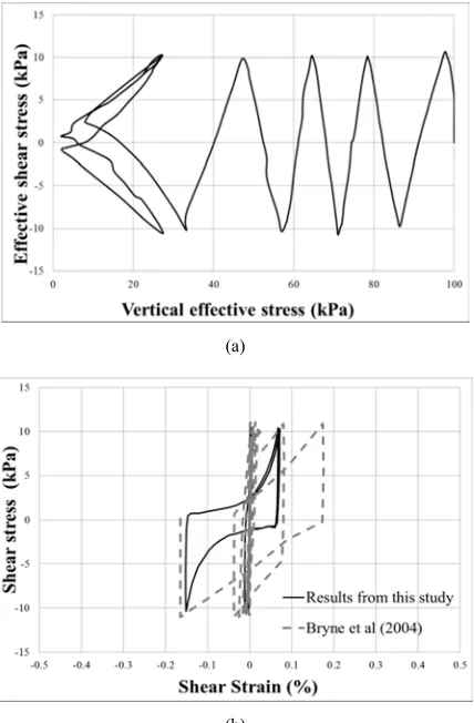
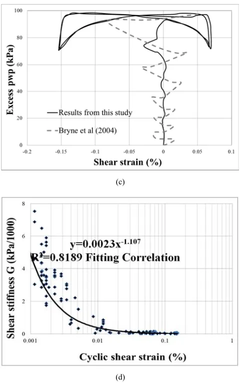
To verify the suitability of proposed model to capture the characteristics of soil liquefaction behavior, an undrained cyclic shear testing is simulated on a cubic sand specimen. The tested soil specimen is assumed to be low to medium dense granular soils with density corresponding to SPT (N1)60

= 10, which can be used to determine the Finn-model parameters [6] as presented in Equations 1 to 5. The dimension of the soil element is a cube with side length of 0.1 m. The initial effective stress is equal to 100 kPa, and the initial horizontal effective confining stress is equal to 100 * 0.5 = 50 kPa, since K = 0.5 (K is the lateral earth pressure

coefficient – the ratio of the horizontal to vertical stress in ground); A cyclic shear stress of 10 kPa is applied on the top of soil specimen. A total of 6 cycles of shear loading is applied after the soil liquefies.

The simulated results are plotted together in Figure 1 include: (a) effective vertical stress vs. effective shear stress; (b) effective shear stress vs. shear strain; (c) EPWP vs. shear strain; (d) shear stiffness degradation vs. shear strain. As shown in Figure 1b, the sudden and significant increase in shear strain indicates the soil element starts to fully liquefy after the 4th cycle, and the soil phase changes from solid to liquid due to the large EPWP generation shown in Figure 1c. In the 5th and 6th cycles, the EPWP reaches 100 kPa, and the vertical effective stress is reduced dramatically as shown in Figure 1a. Figure 1d presents the shear stiffness-cyclic shear strain relationship. A continuous line that fit the points is plotted to show the decreasing trend of the shear stiffness with increasing cyclic shear strain in the soil specimen.

The measured EPWP and shear stress – shear strain results obtained from physical testing are not available to the authors. Hence, to calibrate the fitting parameters and verify the applicability of the “combined” model to properly describe the liquefaction characteristics as mentioned above, Figure 1b and 1c show the simulated results of EPWP and shear stress with cyclic shear strain compared to results from [7, 8]. In [7], the UBSAND model was applied to describe the dynamic behavior of a soil element under simple shear undrained loading condition, and the estimated results are shown in Figure 1a to 1c.

(a)

(c)

(d)

Figure 1. Estimated soil response subjected to undrained cyclic simple shear stress.

The stress states applied in this study for validation purpose are identical to that used in [7]. As shown, results from both studies indicate the testing specimen becomes fully liquefied after the 6th loading cycles. Comparing to the results from [7] in Figure 1b and 1c, the Finn-model parameters (Dr

or SPT (N1)60, C1, C2, C3, and C4) and PL-model parameters

(f and n) are calibrated. In Figure 1b, correlations of cyclic shear stress – strain with loading cycles from both studies match very well, but the shear strain value from [7] increases faster and reaches 0.2% after 5 loading cycles. Hence, this may lead to a smaller estimated deformation for post-liquefaction condition by using the “combined” model.

A similar conclusion can also be made based on Figure 1c. EPWP vs. shear strain correlations from this study and [7, 8] reach a good match, but shear strain increases faster in the first 5 cycles before the specimen becomes fully liquefaction. Data from [7] for plotting Figure 1a and Figure 1d are not available, therefore only the estimated shear stress-shear strain and EPWP-shear strain correlations are compared.

The Finn-model, as used in this study to describe the pre-liquefaction behavior, is the main reason of leading the differences in the shear stress vs. strain correlation and excess PWP vs. shear strain correlation in the initial 5 cyclic loading

cycles of both studies. Based on the validation results in [9], the Finn model normally tends to underestimate the excess pore water pressure and development of cyclic shear strain during the cyclic loading for undrained condition. With the generation of excess pore water pressure reaching approximate 0.6, the soil constitutive model “switches” to PL-model, the predicted shear strain results in both studies start increasing dramatically.

Therefore, above observations indicate the typical liquefaction failure characteristics can be reasonable well captured by simulating a low density granular soil element with the initial vertical effective stress of 100 kPa and cyclic shear stress of 10 kPa. Hence, the capability of the utilized “combined” model for simulating soil liquefaction failure mechanisms is verified, and the fitting parameters can be calibrated based on the comparison results in Figure 1b and 1c.

2.2. Case History Simulation Verification

A verified case history simulation can be used as an unimproved benchmark within this framework to show the initial failure mechanism. Once verified, a comparison can be made between the unimproved and improved performance to show the effectiveness of improvement measures.

2.2.1. Field Structure-Soil Deformation Observations

The analyzed case history corresponds to the typical gravity caisson quay wall section in the Kobe earthquake in 1995, in which both foundation soil and backfill soil are liquefiable [2, 11]. Due to the large movement of quay wall during seismic loading, phenomena of liquefaction such as ground fissures or soil boiling may not be so obvious in the backfill soil immediately close to the quay wall. As recorded in [3, 4], the wall top displaced seaward approximately 4.5 m (exceeding 5 m in a few locations) during the earthquake. The wall settled about 1–2 m and tilted about 4 degrees seaward. No structural damage or crack was observed on the deformed caisson walls along the coastline. Significant deformations in the soils were observed within a zone extending about 25 to 30 m behind the wall. Very limited deformations were observed in the free-field approximately 80 to 100 m away from the caisson wall even though some traces of liquefaction were observed such as sand boiling at this distance. Investigation by divers, as reported in [3, 4], revealed a substantial heaving of a foundation layer at a distance of 2 to 5 m in front of the bottom seaward toe of the caisson.

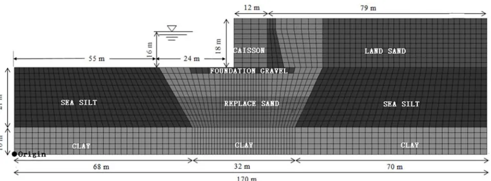
2.2.2. Numerical Model and Analysis

In the current model, the length, height and width of the model are 170 m, 49 m and 10 m, in X, Z, and Y-directions, respectively, based on actual dimensions [3, 4]. The left bottom corner (Z=0) of the model is set as the original point, and the original point is important to locate Point A to H.

and 1 m in the soil zone immediately adjacent to the caisson wall. The average calculation time for one single case is

around 15 hours.

Figure 2. Established model for the simulated case history.

For the constitutive model, the caisson quay wall is modeled as an elastic body, having an interface that allows slippage and separation at the base and the back of the caisson wall. The potentially liquefiable soils are foundation soil and backfill soil, which are both modeled using Mohr-Coulomb failure criteria for static analysis and the “combined” model for dynamic analysis. The other non-liquefiable zones (seabed clay and sea silt zone) are modeled by using Mohr-Coulomb failure criteria in both static and dynamic analysis.

The dynamic input includes two histories of accelerations (m/sec2) in vertical and horizontal directions recorded at a depth of 32 m in the Port Island array [12]. The peak acceleration values were recorded as 0.60g and 0.20g, respectively, as shown in Figure 3. The two time histories of accelerations are applied as the seismic input at the bottom nodes of the model.

Figure 3. Time history of accelerations (cm/sec2_{) (Inagak and Tai, 1996).}

The boundary condition at the sides of the model was achieved using the free-field condition (“FF”) and to minimize wave reflections without using an impractical model [2]. The interface parameters of this model include the normal and shear stiffness, cohesion and friction angle, which are not easily determined in the field and have to be

determined based on the material properties, stress state and relative movement between the two attached materials (the gravel foundation layer and concrete caisson wall). The details can be found in the FLAC3D User’s Manual [2]. A sensitivity study was performed to determine the influence of interface parameters on the deformation of the quay wall (Table 1), and the results indicated that increasing the value of normal stiffness and/or shear stiffness of the thin foundation layer material within a reasonably realistic range could only lead to a slightly decreasing value of deformation of the caisson wall. The influence is limited, less than 5% of the caisson wall’s total deformation. This may indicate that a thin stronger foundation layer underneath the caisson wall only provide limited contribution to reduce the deformation of the caisson wall if the caisson wall were placed on fully liquefied soil. Additional study of the interface issue using more sophisticated models to predict the interface behaviors is recommended to verify the influence of stiffness of the interface materials on global deformation of caisson wall-soil system.

Therefore, based on advised values of FLAC3D (2007), normal stiffness and shear stiffness used in this case are recommended to be 1.00E8 and interface mesh length is 1.5 m, and cohesion as 0. As shown in Table 1, the results indicated that the influence of using different interface parameters on wall displacement and tilting angle is insignificant.

2.2.3. Material Properties

Referring to [3, 4, 11, 13], the backfill soil is 16 m thick of loose hydraulic sand fill over dense clay. A similar granular material used for backfill soil ground was also used as the foundation soil under the caisson wall. The ground water table was about 3 m below the backfill ground surface, and the reported SPT resistance for the backfill soil and foundation soil was 10 to 15 on Rooko Island. Therefore, the estimated relative density and SPT (N1)60 for both foundation

respectively, as reported in [4, 11] and used in [14, 15]. The friction angle for the foundation and backfill soil is 37 degrees, as used by [13]. The seabed clay and sea silt zone are non-liquefiable and assumed to be medium to high density [5]. All zones expect for the caisson wall are assumed to be isotropic, and the permeability values are estimated based on their relative density [16]. The other material properties such as density, permeability, bulk and shear modulus, porosity, cohesion, Poisson’s ratio are estimated based on SPT (N1)60 by using the empirical correlations as

provided by [16] or directly from the published data [13, 15, 20]. As recommended by [16], the geological material damping commonly falls in the range of 2 to 5% of the critical damping ratio. For many non-linear dynamic analyses that involve large strain, only a minimal percentage of damping ratio (e.q., 5%) may be required. Therefore, the local damping of 0.157 is used for all soil zones (Itasca 2007) based on calibration of the case history as presented below. A summary of the soil parameters used in both static and dynamic analysis is presented in Table 1 and 2.

Table 1. Materials properties and model parameters used in static analysis.

Material Model Density (kg/m3) Elastic Modulus (Mpa) Poisson’s ratio Cohesion (Kpa) Friction angle (Deg)

Seabed Clay MC 1550 30 0.33 30 20

Sea silt MC 1550 20 0.33 10 30

Foundation soil MC 1350 15 0.33 10 37

Backfill soil MC 1350 13.7 0.33 10 37

Foundation layer MC 1550 100 0.33 10 40

Caisson Elastic 2800 1300 0.17 - -

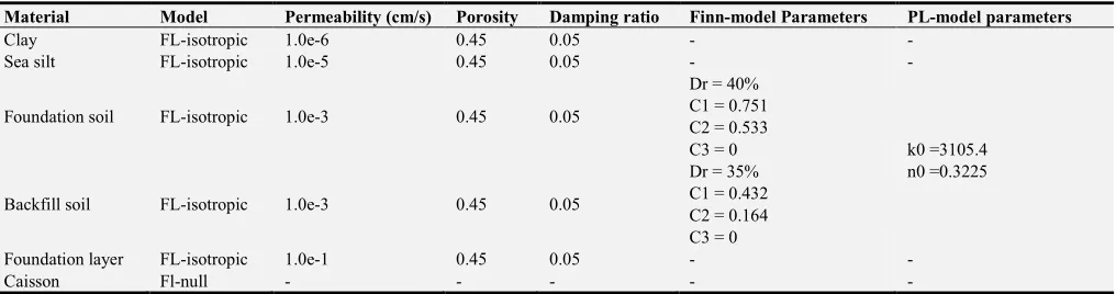
Table 2. Material properties and model parameters used in dynamic analysis.

Material Model Permeability (cm/s) Porosity Damping ratio Finn-model Parameters PL-model parameters

Clay FL-isotropic 1.0e-6 0.45 0.05 - -

Sea silt FL-isotropic 1.0e-5 0.45 0.05 - -

Foundation soil FL-isotropic 1.0e-3 0.45 0.05

Dr = 40% C1 = 0.751 C2 = 0.533

C3 = 0 k0 =3105.4

n0 =0.3225

Backfill soil FL-isotropic 1.0e-3 0.45 0.05

Dr = 35% C1 = 0.432 C2 = 0.164 C3 = 0

Foundation layer FL-isotropic 1.0e-1 0.45 0.05 - -

Caisson Fl-null - - - - -

2.2.4. Estimated Structure – Soil Deformations

The deformed caisson wall–soil deformations with contours of deformation labeled are shown in Figure 4. Figures 4a and 4b show the calculated seaward and vertical displacement at the seaward top corner of the caisson wall is approximately 4.4 m and 2.5 m, respectively. The calculated residual seaward rotation is about 4.3 degrees. The displacement counters show that both surface horizontal and vertical deformation in backfill soil propagate with the increasing distance from the caisson wall. Approaching the right boundary of the model, at around 80 meter from the caisson wall in the backfill soil, the calculated seaward and vertical displacement are less than 0.1 m. This is consistent with the observation over a distance of 100 to 200 m from the back of quay walls [21]. Also, the retained soil immediately behind the caisson wall settled significantly (with the maximum settlement of 2 m).

Moreover, the foundation soil layer was substantially

deformed underneath the seaward edge of the foundation and substantially heaved in from of the toe of the wall, which clearly indicated a reduced bearing capacity of the foundation soil under rotational and lateral movement of the heavy caisson wall. This observation is also consistent with the results presented by [13]. The calculated caisson wall deformations provide good agreement with the field observations [3, 4].

Figure 4. Deformations of the caisson wall-soil system.

2.2.5. Estimated Excess Pore Water Pressure Generation

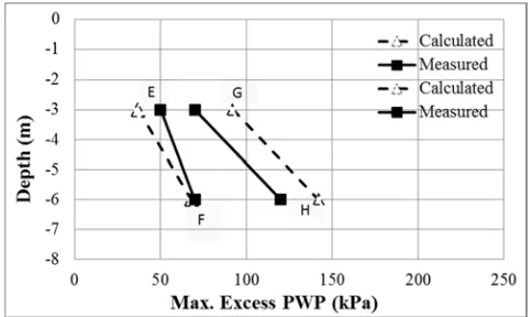
The estimated distribution of EPWP generation in both foundation and backfill soils show consistency with previous studies [3, 4, 13]. References [3] performed a shaking table test on the identical case history presented in Figure 2, and the EPWP results measured at locations as shown in Figure 5. The calculated distributions of maximum EPWP in the foundation and backfill soils from this study are compared to their results in Figure 6. The extensive EPWP generated in both foundation soil and backfill soils, explained the large deformations (settlement and seaward movement) that occurred in both liquefied foundation and backfill soils, and the wall also move seaward and rotated.

Reference [13] analyzed the identical case history using numerical methods, and their results offer a strong qualitative corroboration to the observations on EPWP and deformation patterns of the caisson quay wall, foundation and backfill

soils obtained in [3, 4].

Overall, the generation and distribution of EPWP in both foundation and backfill soils were important to understand the failure mechanism of caisson wall deformation and hence to provide viable liquefaction mitigation. In brief, the EPWP in foundation soil is low because of the dead weight of the caisson wall, which increases initial effective overburden pressure and somewhat protects the replaced sand from being liquefied. The generation and distribution of EPWP in the backfill soil was influenced by the gradual movement of caisson wall with cyclic loading, which didn’t allow a continuous accumulation of EPWP in this region, especially for the soil zones adjacent to the wall. This may explain why there was generally a lack of liquefaction evidence on the surface whereas in the backfill soil further in land here was extensive evidence of liquefaction.

Points A, B, C, and D (Figure 5) are located in backfill soil with a horizontal distance of 20-25 m away from the caisson wall. The depth of A, B, C, and D from the backfill land surface is approximately 4 m, 8 m, 13 m and 16 m based on the scaled dimensions. In the foundation soils, points E and F, G and H were located near the front of the seaward bottom corner and immediately behind the inward corner of the caisson wall, respectively. The depth of points E and G, and F and H is the same, which are 4 and 8 m respectively, below the caisson wall bottom. The maximum EPWP at these points cases were measured and plotted.

Figure 6. Comparisons of the maximum EPWP distribution between the calculated and tested values of the measuring locations.

Accordingly, the locations in the simulated model corresponding to the above points were highlighted, and the EPWP values at these locations were calculated and compared to the measured results. The maximum EPWP value was back calculated based on the difference between the initial PWP prior to dynamic analysis and the maximum PWP ratio from the computation. The calculated initial PWP value and maximum PWP values at point A to H are shown in Table 3, which are compared to the average measured values from cases 2, 6 and 7 from [3 and 4], as presented in Figure 5.

Table 3. Calculated maximum EPWP at the highlighted locations.

ID Coordinates Improved zone Initial PP (kPa) Max PP (kPa) Max Ex. PP (kPa) EPWP ratio

A (110, 46, 5) Backfill 8.8 29.4 20.6 0.71

B (110, 37, 5) Backfill 61.3 107 45.7 0.87

C (110, 28, 5) Backfill 131 262 131 0.79

D (110, 20, 5) Backfill 173 181 8 0.3

E (80, 25, 5) Foundation 217 254 37 1.12

F (80, 20, 5) Foundation 261 329 68 0.76

G (100, 25, 5) Foundation 195 284 92 0.58

H (100, 20, 5) Foundation 261 403 142 0.44

The comparisons are shown in Figure 6 and the general good agreements are received, except for Point G and H, where the calculated max EPWP varied by a factor of 2 comparing with the measured values. Point G and H are located in replaced sand zone, where adjacent to the land sand zone. In this region, the migration of excess PWP between the replace sand and land sand could occur, which could explain why the measured excess PWP was smaller than the estimated values, because migration of PWP is not properly considered in the computation. The calculated PWP ratio values at these various locations agree well with the measured values, and the results properly describe the distribution of EPWP in backfill and foundation soil. The results at Points G and H are not in as good agreement, but still acceptable.

As shown, the backfill soil and the foundation soil in front of the bottom corner of caisson wall suffer more severe liquefaction. The coordinates of Point A to H are determined with accordance to the original point at the left bottom corner of the model. Based on above results, the overall estimated responses in terms of deformations, EPWP distributions are

consistent with the observed behavior [4]. Therefore, the simulated case history, as the framework for the application of ground improvement methods in next phase, is verified. The verification process, which includes both the verification on the soil constitutive model and on the simulated case history based on the field observations and the measured maximum PWP at highlighted locations, shows that the simulated case history is reliable. Therefore, it can be used as the framework to further study the liquefaction triggering mechanisms of the unimproved scenario and evaluate the influences of ground improvement applications.

3. Parametric Study Parameters

Due to the limited computation capacity, only the key design parameters of the vibro-compaction program and level of excitation in terms of peak ground acceleration (PGA) are investigated. The dimension and properties of the caisson quay wall, backfill soil and foundation soil are remained unchanged as reported based on filed observation in [4].

The cross section of the simulated case history is shown in Figure 2. The major analyzed parameters of the improved zone configurations can be specified by the lateral length (L) of improved zone in backfill soil and vertical depth (D) of the improved zone in foundation soil. The testing metrics of the numerical study is presented in Table 4. Both parameters are specified by a ratio with respect to the wall height (H). The improved depth in backfill soil is equal to the full thickness of backfill soil profile. Therefore, the parameters used in this study were L/H = 0.5, 1.0, 1.5, 2.0, 2.5, 3.0 (e.g., 3.0 refers to 3.0*18 m = 54 m away from the caisson wall in backfill soil); D/H = 0.3, 0.6, 0.9, 1.2 (e.g., 1.2 refers to 1.2*18 = 22 m, the full thickness of the foundation soil layer). In this study, the caisson wall height (H) is 18 m and the wall width (W) is 12 m, and both remain unchanged in the parametric study.

Above parameters are within the range of interest for most port structures.

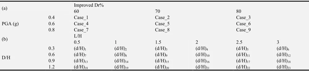
The improved Dr% of the improved soil is 60%, 70%, and 80% with various probing distance of 2.3 m, 2.0 m and 1.7 m (Table 5), respectively, based on the empirical chart for preliminary design [18]. The peak ground accelerations of the input seismic excitation assigned at the bottom node of the model is 0.4g, 0.6g, and 0.8g. Therefore, the testing parametric metrics are shown in Table 4. In part (a) of Table 4, a total of 9 cases are shown by differing in improved Dr% and level of seismic input excitation (PGA); in part (b) of Table 4, which refers to the metrics in one single case, a total of 23 residual displacements are calculated by differing the improvement zone configurations in terms of L/H and D/H ratios as presented above. Therefore, the total number of analyzed cases in this study is 23*9= 317. In addition, the influences of other variables, such as caisson quay wall dimension and weight, seawater water depth, and other in-situ soil parameters, are not included in this study due to the computational limit. However, these variables can be easily studied by following the same process as conducted herein.

Table 4. The conducted parametric study.

(a) Improved Dr%

60 70 80

PGA (g)

0.4 Case_1 Case_2 Case_3

0.6 Case_4 Case_5 Case_6

0.8 Case_7 Case_8 Case_9

(b) L/H

0.5 1 1.5 2 2.5 3

D/H

0.3 (d/H)1 (d/H)2 (d/H)3 (d/H)4 (d/H)5 (d/H)6

0.6 (d/H)7 (d/H)8 (d/H)9 (d/H)10 (d/H)11 (d/H)12

0.9 (d/H)13 (d/H)14 (d/H)15 (d/H)16 (d/H)17 (d/H)18

1.2 (d/H)18 (d/H)19 (d/H)20 (d/H)21 (d/H)22 (d/H)23

3.1. Liquefaction Remediation Using Vibro-Compaction Method

For simplicity, the improved soil properties for foundation soil and backfill soil are assumed to be the same, primarily represented by the Dr% or SPT (N1)60 value. The properties

of caisson wall, seabed clay and silts remain the same as in the unimproved scenario (Table 2). The improved properties

are determined primarily based on SPT (N1)60 value or from

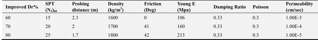
published data or empirical correlations. The empirical correlation between vibration distance and improved Dr% is presented in Figure 7. The improved Dr% data in Table is converted to equivalent SPT blow count using the Tokimatsu and Seed (1984) relationship for granular soils. The improved parameters are mainly estimated based on the published data or empirical correlations [16, 18 and 19].

Table 5. Improved soil properties.

Improved Dr% SPT (N1)60

Probing distance (m)

Density (kg/m3₎

Friction (Deg)

Young E

(Mpa) Damping Ratio Poisson

Permeability (cm/sec)

60 15 2.3 1600 0 106 0.33 0.3 1.00E-3

70 20 2 1700 41 160 0.33 0.3 1.00E-4

80 25 1.7 1800 42 213 0.33 0.3 1.00E-5

3.2. Parameter Sensibility on Quay Wall Displacement

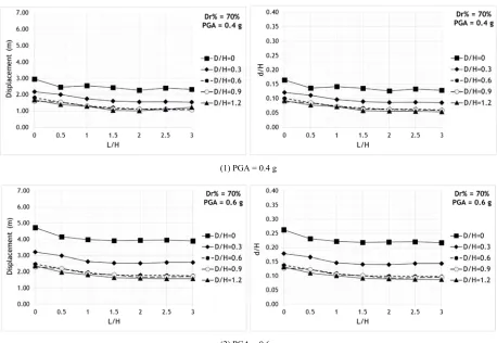
The next challenge to overcome is to present the parametric study results from 315 numerical analyses in a meaningful way. A parameter so-called “Engineering Demanding Parameter or EDP” is needed to describe and quantify the structure response effectively and representatively. According to [23], the seismic performance of gravity caisson quay walls is typically evaluated by the seismic residual displacement of the seaward top corner of the walls. Therefore, the results of this conducted parametric study are summarized in terms of the residual displacement (d) at the seaward top corner of the caisson quay wall; then, the influence of the analyzed parameters can be evaluated on a comparative basis by quantifying their effects on the residual displacement (d).

First, based on the computed residual displacement (d) values, the optimum L/H and D/H values corresponding to the various cases (shown in part (a) of Table 4) differing in improved Dr% and levels of seismic excitation (expressed by PGA) can be found. Then, the effects of the major parameters are discussed with respect to the improved residual displacement magnitude (d) and the normalized residual displacement ratio (d/H). Therefore, the calculated displacement (d) or displacement to wall height ratio (d/H) are investigated against with the key design parameters (L/H and D/H) under the influences of various improved Dr% and seismic excitation levels (PGA) in following sections.

3.3. Optimum Improvement Zone Configurations in Terms of L/H and D/H Values

The optimum L/H and D/H values for all the cases as shown in part (a) of Table 4 are shown in Table 6. The adopted method of determining the critical L/H and D/H values are mainly based on their calculated displacement (d) values and the additional reduction in (d) with the further

increasing in L/H and D/H. The more detailed descriptions of the adopted method can be referred to [24]. In general, two evaluation criteria (1) improvement effectiveness expressed by the improved residual displacement (unit: m) and (2) improvement efficiency (unitless) expressed by the ratio of displacement reduction over improvement effort indicated by the improved zone volume are used to evaluate a remedial plan. This is based on the assumptions that the remedial program cost primarily depends on the volume of improved soil. As an illustration instance, case 7 with improved Dr% = 60% and PGA = 0.8 g is illustrated, and the results of all the other cases are found close to Case 7, and their results are attached in Table 7 in Appendix for reader’s reference. In this study, the specific quay wall height is 18 m and the initial unimproved displacement at the top seaward corner of the caisson quay wall is computed to be 4.7 m (Figure 4).

As seen in Figure 8–(a), the increasing of L/H and D/H leads to a reduction in displacement (d) for all presented curves differing in D/H ratios. However, the reduction magnitude of (d) or the additional benefit becomes less apparent when the value of L/H and D/H equals or exceeds to approximately 2.0 and 0.6, respectively. Therefore, the L/H value of 2.0 and D/H equal of 0.6 is recommended as the optimum improved zone configuration under this specific condition. The reduced residual displacement is predicted to be 2.52 m and the achieved reduction is approximate 62% (1-2.52/6.59=0.62 or 62%). This improved deformation may not be accepted since the improved displacement of 2.52 m is still larger than the repairable limit near collapse of less than 1.8 m under the strong earthquake motion for gravity caisson wall [23]. Therefore, specifying the improved Dr% of 80% and the minimum L/H and D/H values of 2.0 and 0.6 (36 m and 11 m in this case), respectively, is recommended to achieve the improved displacement to be 1.41 m and the reduction percentage to be 80% (1-1.41/6.59=0.8 or 80%).

Table 6. The optimum values of D/H and L/H and the computed displacement (d).

Case ID Improved Dr% PGA (g) L/H D/H d (m) d/H

1 60 0.4 1.5 0.6 1.37 0.08

2 70 0.4 1.5 0.6 1.13 0.06

3 80 0.4 1.5 0.6 0.74 0.04

4 60 0.6 1.5 0.6 2.03 0.11

5 70 0.6 1.5 0.6 1.81 0.10

6 80 0.6 1.5 0.6 1.14 0.06

7 60 0.8 2.0 0.6 2.52 0.14

8 70 0.8 2.0 0.6 2.31 0.13

9 80 0.8 2.0 0.6 1.41 0.08

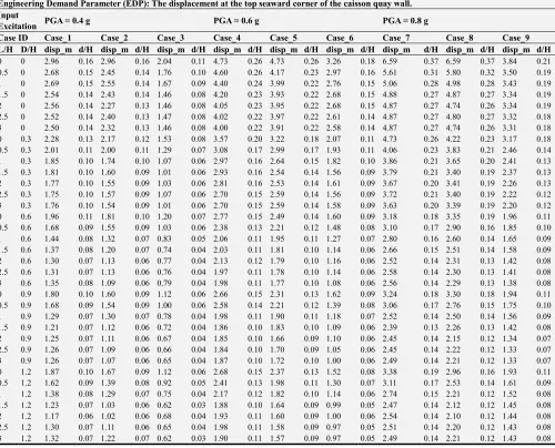
Table 7. Overall parametric study results.

Engineering Demand Parameter (EDP): The displacement at the top seaward corner of the caisson quay wall. Input

Excitation PGA = 0.4 g PGA = 0.6 g PGA = 0.8 g

Case ID Case_1 Case_2 Case_3 Case_4 Case_5 Case_6 Case_7 Case_8 Case_9

L/H D/H disp_m d/H disp_m d/H disp_m d/H disp_m d/H disp_m d/H disp_m d/H disp_m d/H disp_m d/H disp_m d/H

0 0 2.96 0.16 2.96 0.16 2.04 0.11 4.73 0.26 4.73 0.26 3.26 0.18 6.59 0.37 6.59 0.37 3.84 0.21

0.5 0 2.68 0.15 2.45 0.14 1.76 0.10 4.60 0.26 4.17 0.23 2.97 0.16 5.61 0.31 5.80 0.32 3.50 0.19

1 0 2.69 0.15 2.55 0.14 1.67 0.09 4.40 0.24 3.99 0.22 2.76 0.15 5.06 0.28 4.98 0.28 3.43 0.19

1.5 0 2.54 0.14 2.43 0.14 1.46 0.08 4.20 0.23 3.93 0.22 2.68 0.15 4.88 0.27 4.87 0.27 3.34 0.19

2 0 2.56 0.14 2.27 0.13 1.46 0.08 4.05 0.23 3.95 0.22 2.68 0.15 4.87 0.27 4.74 0.26 3.34 0.19

2.5 0 2.52 0.14 2.40 0.13 1.47 0.08 4.02 0.22 3.97 0.22 2.61 0.14 4.87 0.27 4.80 0.27 3.32 0.18

3 0 2.50 0.14 2.32 0.13 1.46 0.08 4.00 0.22 3.91 0.22 2.58 0.14 4.87 0.27 4.74 0.26 3.31 0.18

0 0.3 2.28 0.13 2.17 0.12 1.53 0.08 3.57 0.20 3.22 0.18 2.07 0.11 4.73 0.26 4.22 0.23 3.17 0.18

0.5 0.3 2.01 0.11 2.00 0.11 1.29 0.07 3.08 0.17 2.99 0.17 1.93 0.11 4.06 0.23 3.83 0.21 2.46 0.14

1 0.3 1.85 0.10 1.74 0.10 1.07 0.06 2.97 0.16 2.64 0.15 1.82 0.10 3.86 0.21 3.65 0.20 2.41 0.13

1.5 0.3 1.81 0.10 1.60 0.09 1.01 0.06 2.93 0.16 2.54 0.14 1.56 0.09 3.79 0.21 3.40 0.19 2.37 0.13

2 0.3 1.77 0.10 1.55 0.09 1.03 0.06 2.81 0.16 2.53 0.14 1.61 0.09 3.67 0.20 3.41 0.19 2.26 0.13

2.5 0.3 1.75 0.10 1.57 0.09 1.07 0.06 2.70 0.15 2.59 0.14 1.56 0.09 3.72 0.21 3.40 0.19 2.22 0.12

3 0.3 1.76 0.10 1.54 0.09 1.01 0.06 2.70 0.15 2.59 0.14 1.58 0.09 3.63 0.20 3.39 0.19 2.20 0.12

0 0.6 1.96 0.11 1.81 0.10 1.20 0.07 2.77 0.15 2.49 0.14 1.60 0.09 3.18 0.18 3.35 0.19 1.96 0.11

0.5 0.6 1.68 0.09 1.55 0.09 1.03 0.06 2.38 0.13 2.21 0.12 1.48 0.08 3.10 0.17 2.90 0.16 1.85 0.10

1 0.6 1.44 0.08 1.32 0.07 0.83 0.05 2.06 0.11 1.95 0.11 1.27 0.07 2.80 0.16 2.60 0.14 1.65 0.09

1.5 0.6 1.37 0.08 1.20 0.07 0.74 0.04 2.03 0.11 1.81 0.10 1.14 0.06 2.66 0.15 2.51 0.14 1.58 0.09

2 0.6 1.30 0.07 1.13 0.06 0.77 0.04 2.13 0.12 1.79 0.10 1.16 0.06 2.52 0.14 2.31 0.13 1.42 0.08

2.5 0.6 1.31 0.07 1.13 0.06 0.76 0.04 1.97 0.11 1.78 0.10 1.14 0.06 2.58 0.14 2.30 0.13 1.41 0.08

3 0.6 1.35 0.08 1.09 0.06 0.79 0.04 1.98 0.11 1.77 0.10 1.08 0.06 2.56 0.14 2.29 0.13 1.38 0.08

0 0.9 1.80 0.10 1.60 0.09 1.12 0.06 2.66 0.15 2.31 0.13 1.62 0.09 3.24 0.18 3.30 0.18 1.94 0.11

0.5 0.9 1.68 0.09 1.54 0.09 1.00 0.06 2.58 0.14 2.21 0.12 1.39 0.08 3.06 0.17 2.76 0.15 1.75 0.10

1 0.9 1.29 0.07 1.30 0.07 0.78 0.04 1.98 0.11 1.90 0.11 1.18 0.07 2.52 0.14 2.50 0.14 1.56 0.09

1.5 0.9 1.21 0.07 1.12 0.06 0.72 0.04 1.86 0.10 1.83 0.10 1.09 0.06 2.39 0.13 2.26 0.13 1.42 0.08

2 0.9 1.25 0.07 1.11 0.06 0.67 0.04 1.85 0.10 1.66 0.09 1.10 0.06 2.45 0.14 2.15 0.12 1.34 0.07

2.5 0.9 1.26 0.07 1.09 0.06 0.66 0.04 1.84 0.10 1.70 0.09 1.05 0.06 2.45 0.14 2.22 0.12 1.33 0.07

3 0.9 1.26 0.07 1.07 0.06 0.65 0.04 1.87 0.10 1.72 0.10 1.00 0.06 2.49 0.14 2.21 0.12 1.33 0.07

0 1.2 1.87 0.10 1.67 0.09 1.12 0.06 2.68 0.15 2.37 0.13 1.52 0.08 3.38 0.19 2.96 0.16 1.93 0.11

0.5 1.2 1.62 0.09 1.39 0.08 0.92 0.05 2.41 0.13 1.98 0.11 1.30 0.07 3.11 0.17 2.53 0.14 1.61 0.09

1 1.2 1.38 0.08 1.29 0.07 0.75 0.04 2.17 0.12 1.82 0.10 1.14 0.06 2.74 0.15 2.21 0.12 1.52 0.08

1.5 1.2 1.23 0.07 1.03 0.06 0.62 0.03 1.88 0.10 1.64 0.09 0.99 0.05 2.47 0.14 2.12 0.12 1.45 0.08

2 1.2 1.17 0.06 1.02 0.06 0.68 0.04 1.93 0.11 1.60 0.09 1.00 0.06 2.54 0.14 2.10 0.12 1.44 0.08

2.5 1.2 1.30 0.07 1.11 0.06 0.65 0.04 1.98 0.11 1.58 0.09 0.97 0.05 2.51 0.14 2.20 0.12 1.43 0.08

3 1.2 1.32 0.07 1.22 0.07 0.62 0.03 1.90 0.11 1.57 0.09 0.97 0.05 2.49 0.14 2.21 0.12 1.43 0.08

3.3.1. Improvement Zone Length (L/H) in Backfill Soil

The effects of the improvement zone lateral length to wall height ratio (L/H) on the improved residual displacement are shown in Figure 9 for the improved Dr% of 70% under three examined PGA values. For all D/H values, increasing the improvement zone length (L) in the backfill soil or the L/H value can reduce the residual displacement of the caisson wall. However, when L/H values exceeds 1.5 to 2.0, the influences of further increasing L/H or improving additional backfill soil beyond this distance of 1.5 to 2.0 times of the quay wall height become less obvious for the examined range of D/H values.

3.3.2. Improvement Zone Depth (D/H) in Foundation Soil

The effects of the improvement zone vertical depth to wall height ratio (D/H) on the improved residual displacement are shown in Figure 10 for the improved Dr% of 70% under three examined PGA values. For all L/H values, increasing the improved zone depth (D) in the foundation soil or the D/H value can decrease the residual displacement of the caisson wall, and the reduction magnitude also depends on

the applied PGA and improved Dr%. However, when D/H value exceeds 0.6, the influences of further increasing D/H becomes less significant for the examined range of L/H values.

3.3.3. Improved Dr% and Seismic Excitation Level (PGA)

Based on the optimum improvement zone configuration results presented in Table 6, these results are plotted against with their corresponding improved Dr% under the various examined levels of excitation (PGA) in Figure 11. As seen within the typical range of improved Dr% (from 60% to 80% analyzed in this study) for the vibro-compaction method, increasing the improved Dr% or compacting with a closer probing distance would result in the reduced seismic deformation a given level of seismic excitation expressed by PGA. Also, the higher level of excitation expressed by PGA would also lead to a larger improved residual displacement for a given improved Dr% value.

3.3.4. Overall Parameter Sensitivity

the most sensitive remedial design parameters affecting the improved residual displacement of caisson quay wall under a level of excitation is the improved zone configuration (expressed by D/H) in foundation soil, and the second is the improved zone configuration (expressed by L/H) in backfill soil. Especially under the intensive shaking (comparing Figure 10-3 and 9-3), increasing D/H value is more apparent than increasing L/H on the displacement reduction. This observation also agrees well with the conclusion by [3] that effect of improving foundation soil on the deformation of caisson wall is approximately two times of that by improving backfill soil. The effect of improved Dr% on improved deformation becomes slightly less obvious with the increasing in excitation levels (in Figure 11). The level of excitation also influences the improved displacement largely (in Figure 11). Therefore, specifying the designed earthquake motion is a critical step in remedial design to ensure that whether the improved performance satisfies the specified performance grade.

However, the parametric study above is for a quay wall of H = 18 m and W = 12 m, and the soils in model are following the description in [3], where both foundation soil and backfill soil are liquefiable with initial SPT (N1)60 of 10

to 15. Furthermore, the above results under various scenarios with different wall height and width, in-situ soil properties and thickness, and frequency of excitations should be also studied by following the similar method as adopted in this study.

(1) Displacement (m)

(2) d/H ratio

Figure 8. Calculated residual displacements with L/H and D/H ratio for case 7.

(1) PGA = 0.4 g

(3) PGA = 0.8 g

Figure 9. Effect of L/H ratio in backfill soil (Dr% = 70%).

(1) PGA = 0.4 g

.

(2) PGA = 0.6 g

(3) PGA = 0.8 g

Figure 11. Effect of improved Dr%.

3.4. Procedure for Evaluating Improved Wall Displacement

As mentioned earlier, the numerical analysis is particular useful for optimizing the remedial program using ground improvement based on Performance-Based Design method [23]. However, performing numerical analysis normally requires a high level of engineering and reasonable amount of effort. It is not always easy to apply for routine engineering practice. To overcome this problem, a simplified procedure is necessary for evaluating the improved seismic deformation with a given improvement design features in the routine design practice.

A similar method has been proposed to quickly access the failure model and deformation magnitude of the gravity type quay wall [1], remediation effect was not incorporated in this method. The results of above presented parametric study offer a basis to establish such a method incorporating the influence of soil improvement by the vibro-compaction method on improved seismic deformation prediction.

Given the improved length and depth in liquefiable soil behind and below the caisson wall and the specified Dr% or SPT (N1)60, a simple procedure can be developed for

predicting the improved deformation of gravity type caisson wall that is similar to the wall described in [1]. The flow chart for the simplified procedure is shown in Figure 12. In this procedure, the improved residual displacement can be evaluated with respect to the analyzed parameters in the order of its sensitivity to the improved deformation, as presented in previous section. As the first step, a rough

estimation is made based on the improved zone configuration in Figure 9 and 10. Then, the correction for improved relative density is applied based in Figure 11. As the final step, the estimation in given after the correction for the design earthquake motion can be expressed by PGA in Figure 11.

Figure 12. Proposed procedure to evaluate the improved quay wall displacement.

4. Conclusion

The improved displacement of gravity caisson quay walls was studied analytically within a framework of well-calibrated case history through a parametric study by varying the improved zone configuration, improved Dr% and level of excitation. A set of optimum designs in terms of improved zone configurations are found by differing improved Dr% and level of excitations. The conclusions are applicable for the high caisson quay wall with wall height of 18 m and width of 12 m, and the presented soil conditions described in Inagak et al. (1996). The overall parametric study results are shown in Appendix for reader’s reference.

in the level of excitation in terms of PGA also largely increase the improved deformation while all other parameters remain constant.

Based on the parametric study, a simple procedure of estimating the improved residual deformation of caisson quay wall is also proposed. The applicability of the proposed procedure should be further confirmed by case history data. Also, some other parameters such as quay wall dimensions and weight, in-situ unimproved soil conditions and earthquake loading frequency should be further studied by following the similar method adopted in this study.

Above analyses improve our understanding of the complex improved seismic behavior and enhance the engineering judgment in applying liquefaction mitigation to the gravity type caisson quay wall on the liquefiable soil. This is probably one of the most significant contributions that one can expect from this study.

Acknowledgements

This study was funded by the Strategic Highway Research Program 2 of The National Academies and China Geological Survey Projects (Grant No. 1212011140016 and No. DD20160273). The opinions, findings and Conclusions presented here are those of authors and do not necessarily reflect those of the research sponsor.

References

[1] Ichii, K., Iai, S., Sato, Y., Liu, H., 2002, “Seismic Performance Evaluation Charts for Gravity Type Quay Walls,” Structural Engineering and Earthquake Engineering, JSCE, Vol. 19, No. I, 21 – 31.

[2] Itasca. 2007. Fast Lagrangian Analysis of Continua, Users’ manual, MN: Itasca.

[3] Iai, S., and Sugano, T. 2000, “Shaking table testing on seismic performance of gravity quay walls,” Proceedings of 12th World Conference on Earthquake Engineering, Aug 1-6. [4] Inagak H, Iai S, Sugano T, Yamazaki H, Inatomi T. 1996,

“Performance of caisson type quay walls at Kobe port,” Special Issue of Soils and Foundations 1996; 119-136. [5] Alam, M. J., Towhata, I., Wassan, T. H. 2005, “Seismic

behavior of a quay wall without and with a damage mitigation measure,” GSP 133 Earthquake Engineering and Soil Dynamics.

[6] Martin, G. R., Finn, W. D. L., and Seed, H. B. 1975, “Fundamentals of liquefaction under cyclic loading,” Journal of the Geotechnical Engineering Division, ASCE, 101 (GT5): 423-438.

[7] Bryne, P., Park, S. S., Beaty, M., Sharp, M., Gonzalez, L., Abdoun, T. 2004, “Numerical modeling of liquefaction and comparison with centrifuge tests,” Can. Geotechnical Journal, 41: 193-211.

[8] Bryne, P. M. 1991, “A cyclic shear-volume coupling and pore pressure model for sand,” In Proceedings of the 2nd International Conference on Recent Advances in Geotechnical

Earthquake Engineering and Soil Dynamics, St. Louis., Mo., 11-15, March. Vol. 1, pp. 47-55.

[9] Arablouei, A., Ghalandarzadeh, A., Mostafagharabaghi, A. R., Abedi, K. (2011). “A numerical study of liquefaction induced deformation on caisson-type quay wall using a partially coupled solution.” J. of Offshore Mechanics and Arctic Engineering, 133, 021101-1–021101-9.

[10] Chu, J., Varaksin, S., Klotz, U., and Menge, P. (2009). “State of the Art Report: Construction Processes.” Proc. of 17th Int. Con. on Soil Mechanics and Geotechnical Engineering, Alexandria, Egypt, October 5-9, 2009.

[11] Finn, W. D., Bryne, P. M., Evans,. S, Law, T. 1996, “Some geotechnical aspects of Hyogo-ken Nanbu (Kobe) earthquake of January 17, 1995,” Can. Journal of Civil Engineering 1996; 23: 778-796.

[12] Iwasaki, Y., Tai, M. 1996, “Strong motion records at Kobe Port Island,” Soils Foundations (Special issue on geotechnical aspects of the January 17, 1995 Hoogoken-Nambu earthquake), 1, 29-40.

[13] Dakoulas, p., Gazetas, G. 2008, “Insight into seismic earth and water pressures against caisson quay wall,” Geotechnique, 58, No. 2, 95 -111.

[14] Alyami, M., Wilkison, S. M., Rouainia, M., Cai, F. 2007, “Simulation of seismic behavior of gravity quay wall using a generalized plasticity model,” Proceedings of 4th International Conference on Earthquake Geotechnical Engineering, June 25 -28, 2007.

[15] Alyami, M., Rouainia, M., Wilkison, S. M. 2009, “Numerical analysis of deformation behavior of quay walls under earthquake loading,” Soil Dynamics and Earthquake Engineering, 29, pp 535-536.

[16] Look, B., 2007, Handbook of Geotechnical Investigation and Design Tables, Taylor & Francis, London, UK.

[17] Andresen, L., Jostad, H. P., Andresen, K. 2011, “Finite element analyses applied in design of foundations and anchors for offshore structures.” International Journal of Geomechanics, Vol. 11, No. 6, 417-430.

[18] Elias, V., Welsh, J., Wareen, J., Lukas, R., Collin, J., Berg, R., 2006, “Ground improvement methods: Reference Manual – Volume I,” NHI Course No. 13204, Federal Highway Administration.

[19] Chen, Y. M., D. P. Xu, FLAC/FLAC3D Fundamentals and Examples, Waterpub, Inc., Beijing, 2007. (In Chinese) [20] Taiyab, M., Alam, M., Zbedin, M., 2012, “Dynamic

Soil-Structure of Gravity Quay Wall and Effect of Densification in Liquefiable Sites,” International Journal of Geomechanics, (Accepted).

[21] Ishihara, K. 1997, Terzaghi oration: Geotechnical aspects of the 1995 Kobe earthquake, Proc. 14th Conf. Soil Mech. Foundation Engineering, Hamburg 4, 2047-2073.

[22] PIANC: Seismic Design Guidelines for Port Structures, Balkema 474 p, 2001.