Vol. 2 Issue 3, March - 2016
Slope Stability Analysis: Case Study
Meftah Ali
Civil Engineering, Sidi Bel Abbés University, Algeria
Abstract — This research presents an analysis of the problems of slope stability, by classical methods, and the finite element method, which uses the resistance reduction technique for calculating safety factor. Modeling in two dimensions of a real slope, gives us different results, the methods used for static analysis and pseudo static under different loads effect as road traffic, the water level, and the earthquake. The study was made on a slope located in the municipality of Mazouna, right on the national road 90 town of Relizane, Algeria.
Keywords— classical methods; finite element methods; safety factor; static; pseudo static.
I. INTRODUCTION
Technicians calculate the safety factor to evaluate slope stability by conventional methods or by the finite element method despite the differences between the results of safety factor. Classical methods use expression Mohr-Coulom for determining the shear stress along the sliding surface. Fellenius [1] .in 1927 introduced the first method that takes the Swedish name, it assumes that the slip line is circular, and neglects the efforts inter slice Janbu [2]. In 1954 proposes a hypothesis on the line thrust so is considered the force and moment equilibrium of a typical vertical slice and the slip line in the vicinity of the lower third of the vertical slice height, in 1955 Bishop [3]. Has assumed that the sum of the vertical forces in a single tranche is zero, this condition makes the application of the formula is very easy, Spencer [4] .in 1967, is based on the assumption of direction inter slice efforts to the safety factor calculation .Morgenstern and Price [5]. In 1965 assumes a function of inter slices forces and inclination of efforts inter slices may vary by an arbitrary function.The perturbation method in 1974, Raulin et al. [6]. The idea is to give an approximate value or that disrupts the normal force by multiplying it by a known term, Sarma [7] .in 1973 offers horizontal acceleration factor as a safety measure a two-dimensional slope.
II. FINITE ELEMENT METHOD
The finite element method allows determining the forces and deformations in any massif, taking into account the progressive rupture and calculating the average safety factor, along with specific elements of the sliding surface. However its use natural slopes is still the domain of the common practice because it requires precise knowledge of two parameters which are most of the time unknown to natural slopes: the original and the exact behavior of state law materials.
In addition, its implementation is very complex and demands in digital level, significant computer technology. A. Benaissa, 2003 [8].
In general, there are two approaches to the analysis of slope stability by finite element method, the first is to increase the load of gravity, and the second is to reduce the shear parameters is a deterministic method based on reducing the friction angle or
cohesion for calculating safety factor. A. Meftah, 2013 [9].
III. PSEUDO STATIC MÉTHOD
This method is derived from the classical method of analysis of static stability of a sloping circular rupture, it is based on the introduction of a force applied to the center of gravity of the massif studied or each soil of the slices component and of intensity equal to its weight or that of each of treated soil slices multiplying by a coefficient of seismic acceleration. The principle of pseudo-static approach is to model the seismic action by an equivalent acceleration that takes into account the probable reaction slope of massive, static nickname efforts are represented by two coefficients Kh and Kv ± called seismic coefficients for characterizing respectively the horizontal components runs downstream and vertical down or bottom of the slope P made massive strength.
IV. ALGERIAN EARTHQUAKE REGULATIONS RPA99
VERSION 2003:
Algerian earthquake regulations, [10] (RPA99 version 2003) is based on several elements:
Division of the territory into several earthquake zones, within which is defined a seismic acceleration;
Consideration of the geological formations that undergo seismic acceleration;
Characterization of the degree of acceptable risk by type of building;
Calculations based on the pseudo-static approach are an acceptable model for the needs of the practice.
experimental observations in so far as the conditions prevailing during an earthquake (seismic acceleration, soil shear strength, pore pressure, etc.) are unknown. It is then relatively easy to calibrate the design parameters so that the results are consistent with observations. The calculation of pseudo-static quilibre should be seen as an adaptation of calibrated calculation methods are not able to take into account all of the phenomena occurring during an earthquake and whose experimental validation remains partial.
Prendre en compte dans un calcul de stabilité sismique des pentes : Kh = 0.5A (%g), Kv = ± 0,3 Kh
c'b + (w - ub)tanφ' 1 + tanαtanφ'
cosα Fs
Fs = (1)
YG- Y w sinα + k (cosα -h ) + kv
R
V. MODELING OF THE SLOPE BY CLASSICS METHODS
Fig. 1. General configuration of the analyzed slope.
Fig. 2. Part of the Site begins to move. [11]. C.T.T.P,
VI. CALCULATED AND RESULTS BY CLASSICS METHODS
Table I. THE GEOTECHNICAL CHARACTERISTICS OF SOIL
Layers
Gravity Humid weight in
(Kn/ M3)
Undrained Cohesion
(Kpa)
Friction Angle in Degree
The Backfill
Layer 19 20 15 °
The Altered
Marl Layer 18 13 17 °
The Own
Marl Layer 21 146 14 °
Stop (gabion)
21 10 35 °
A. Calculations of Static Stability
Table II. SAFETY FACTORS CALCULATED ACCORDING TO (K = 0)
Condition Méthod FS
Circular failure
FS No-circular failure
Without water
Bishop 1.34 1.65
Janbu 1.10 1.30
Ordinary 1.21 1.32
Morgenstern-Price
1.20 1.21
Spencer 1.25 1.41
GLE 1.15 1.21
With water
Bishop 1.28 1.58
Janbu 1.10 1.21
Ordinary 1.15 1.23
Morgenstern-Price
1.05 1.13
Spencer 1.18 1.30
GLE 1.07 1.01
Table II. The results obtained for the analysis of the static stability, it may be noted that for the conditions with water and without water, the safety factors are greater than 1 therefore, theoretically the slope is stable. These results tell us a stability of the slope. Good agreement was observed between the different results obtained in this analysis A, Meftah, 2015 [12
].
B. Calculation of the Pseudo static Stability
Vol. 2 Issue 3, March - 2016
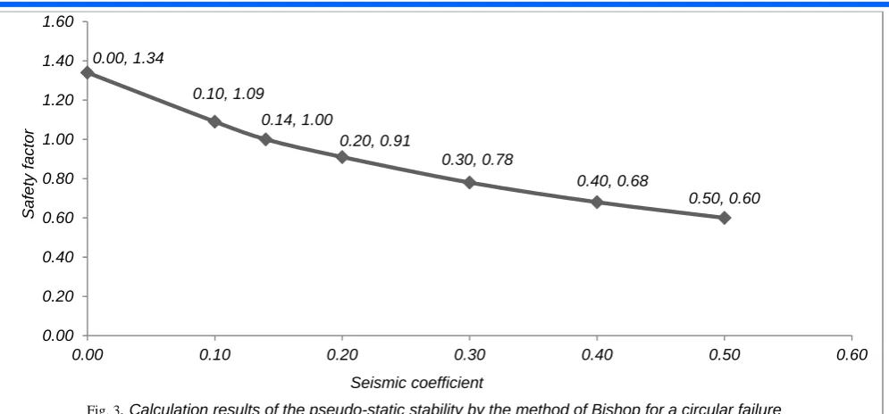
Based on the above analysis of the pseudo static stability, and for circular failure surfaces calculated by the method of Bishop, it was found that the seismic
limit coefficient Kh is of the order of 0.14, the higher seismic coefficients at this value have a safety factor of less than 1, and therefore the slope is unstable.
The figure 4: Represents the results of analyzes of the pseudo-static stability in non-circular failure surface by the method of Bishop
Analyses of the pseudo-static stability performed at the previous slope confirm seismic instability of this slope for non-circular failure surfaces calculated by the method of Bishop, it was found that the seismic coefficient Kh limit is of the order of 0.29, the safety factor Fs is less than 1.
Table III.Analysis of the pseudo static stability by Sarma method .
Form of failure
Horizontal seismic coefficient
Safety factor
Circular failure
0.00 1.15 Static 0.06 1.00 Critical No
Circular failure
0.00 1.29 Static
0.13 1.00 Critical 0.00, 1.34
0.10, 1.09
0.14, 1.00
0.20, 0.91
0.30, 0.78
0.40, 0.68
0.50, 0.60
0.00 0.20 0.40 0.60 0.80 1.00 1.20 1.40 1.60
0.00 0.10 0.20 0.30 0.40 0.50 0.60
Sa
fety
factor
Seismic coefficient
Fig. 3. Calculation results of the pseudo-static stability by the method of Bishop for a circular failure surface
0.00, 1.65
0.10, 1.37
0.20, 1.14
0.29, 1.00
0.30, 0.98
0.40, 0.86
0.5, 0.76
0.00 0.20 0.40 0.60 0.80 1.00 1.20 1.40 1.60 1.80
0.00 0.10 0.20 0.30 0.40 0.50 0.60
Sa
fety
factor
Seismic coefficient
Fig. 4. Results of analyzes of the pseudo-static stability non-circular failure surface by the method
The results obtained with the method of Sarma contain a horizontal seismic coefficient equal to 0.06 for a safety factor Fs is equal to 1 in the case of a failure surface circulaire.et a horizontal seismic coefficient equal to 0.13 for a safety factor Fs equal to 1, table III shows the results obtained.
Table IV. Analysis of the pseudo static stability RPA99 modified in 2003
Form of failure
Horizontal seismic coefficient
Vertical seismic coefficient
Safety factor
Circular
failure 0.13
+0.04 0.98
-0.04 0.99
The analysis of the pseudo-static stability RPA99 modified in 2003 shows the seismic instability of the slope for horizontal seismic coefficient Kh = 0.13 and a vertical seismic coefficient Kv = ± 0.04, these results show that the influence of Kv negligible.
VII. CALCULATIONANDRESULTSFINITE ELEMENT
A. Calculations of static stability (SAS-FEM)
The results of the static safety factor calculations for a non-circular failure surface are present in the following table. A, Meftah, 2016 [13]:
Table V. Analysis of static stability by SAS-FEM
Safoty factor
Without water 1.68
With water 1.2
B. Calculation of the pseudo-static stability
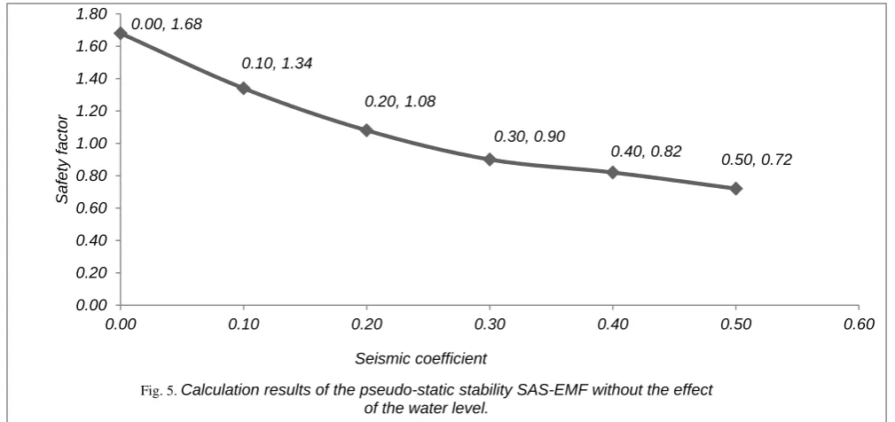
The figure 5: shows the results of calculations of the pseudo static stability by finite element method SAS-EMF without the effect of the water level.
Discussion:
1) Table V shows the results of calculations that distinguish both cases, the first records a 1.68 value of safety factor without the effect of the water level. The second case is introduced the effect of the water level where finding a safety coefficient value is 1.2, the Failure surface of both cases is non-circular, so can be said that the slope remains stable in both case aroused.
2) The analyzes of the pseudo static stability by finite element method without the effect of the water level , the seismic coefficient Kh limit is 0.24, higher seismic coefficients to this value a safety factor of
Less than 1, so in this part the slope is principled goes through three phases, the first where we will find the stable slope that is to say, the higher safety factor than 1, unstable for a lower safety factor 1, and the critical case for equal to1 safety factor
0.00, 1.68
0.10, 1.34
0.20, 1.08
0.30, 0.90
0.40, 0.82
0.50, 0.72
0.00 0.20 0.40 0.60 0.80 1.00 1.20 1.40 1.60 1.80
0.00 0.10 0.20 0.30 0.40 0.50 0.60
Sa
fety
factor
Seismic coefficient
Vol. 2 Issue 3, March - 2016
Discussion:
From analysis of the pseudo static stability by finite element method (SAS-GEF) and under the effect of the web, the seismic coefficient limit is 0.08. the higher seismic coefficients at this value have a safety factor of less than 1.
C. Analysis by RPA 99 modified in 2003
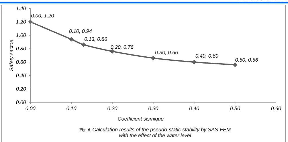
For horizontal seismic coefficient Kh = 0.13, and under the effect of traffic loads and the effect of the water level, the SAS-FEM software gives us a safety factor Fs = 0.86, so the theory is unstable slope.
VIII. CONCLUSIONSANDPROSPECTS
The analysis of the stability of the slope Mazouna gives different results in the calculation of safety factor, that these methods are not based on the same assumptions. In geotechnical practice, there are several sources of uncertainty in the analysis of slope stability, for example, spatial uncertainty (topography and stratigraphy, etc ...) and input data uncertainties (soil characteristics, soil properties in situ, etc …
Among the parameters influencing the safety factor, particularly note the soil shear parameters (cohesion and friction angle), but also the level of the table if present. Their knowledge is accurately known if we want to get results from significant and representative calculations of the state of earth structures.
Using the finite element method is a very important step for the practical study of the slopes.
Following this model, there are many prospects appear either at modeling or level calculation method.
The level of modeling, it is recommended to model the gradient three-dimensional "3D" to reproduce the mechanism observed in the field, and to conclude the importance of the third dimension.
At calculation method, it is recommended that analyzes the dynamic method by using a response spectrum of an earthquake, to reach a state closest to reality.
REFERENCES
[1] W. Fellenius, 1927. earth static calculations with friction and cohesion (adhesion), and assuming circular cylindrical sliding surfaces, Ernst & Sohn, Berlin.
[2] N. Janbu, 1954. Applications of Composite Slip Surfaces for Stability Analysis. In Proceedings of the European Conference on the Stability of Earth Slopes, Stockholm, Vol. 3,p p. 39-43.
[3] W. Bishop, 1955.The use of the slip circle in the stability analysis of slopes. Geotechnique 5(1), p p 7–17.
[4] E. Spencer, 1967. A Method of Analysis of Embankments assuming Parallel Interslice Forces. Geotechnique, Vol 17 (1), pp. 11-26.
[5] N. R. Morgenstern, and V. E. Price, 1965. The Analysis of the Stability of General Slip Surfaces. Geotechnique, Vol.15, pp. 79-93
[6] N .P. RAULI, G. ROUQUES, et L. A. TOUBO, 1974, Calcul de la stabilité des pentes en rupture non circulaire, Rapp. Rech. LPC, 36, juin 1974, 106 p.
[7] S.K.Sarma,1973. Stability Analysis of Embankments and Slopes. Geotechnique, Vol. 23 (3), pp. 423-433.
[8] A, Benaissa, 2003. "Glissements de terrains" calcul de stabilité. OPU, 95p
[9] A. Meftah, 2013. "L’utilisation de la méthode des éléments finis et les méthodes classiques pour l’analyse statique et pseudo statique de la stabilité des talus" mémoire de Magister, Université de Saida, Algérie, 2013, 127 p.
0.00, 1.20
0.10, 0.94
0.13, 0.86
0.20, 0.76
0.30, 0.66
0.40, 0.60
0.50, 0.56
0.00 0.20 0.40 0.60 0.80 1.00 1.20 1.40
0.00 0.10 0.20 0.30 0.40 0.50 0.60
Sa
fety
sacto
e
Coefficient sismique
[10] RPA. 1999 (Version 2003). "Règles Parasismiques Algérienne ", 89 p.
[11] CTTP. juin 2007. Étude de confortement du glissement sur R N 90 au pk 75+700 Rapport géotechnique final.
[12] A.Meftah, 2015. "Static analysis and pseudo static slope stability", International Journal of Civil, Environmental, Structural, Construction and Architectural Engineering, waste, Vol: 9, No: 6, 2015, pp. 658 - 661.
![Fig. 2. Part of the Site begins to move. [11]. C.T.T.P, (2007)](https://thumb-us.123doks.com/thumbv2/123dok_us/8358469.1670079/2.595.58.277.500.746/fig-site-begins-c-t-t-p.webp)