Optimal Experimental Design for
Semiconductor Lifetime Mission Profile Testing
Stefan SchrunnerKAI – Kompetenzzentrum Automobil- und Industrieelektronik GmbH
Villach, Austria [email protected]
Olivia Bluder
KAI – Kompetenzzentrum Automobil- und Industrieelektronik GmbH
Villach, Austria [email protected]
Jürgen Pilz
Alpen-Adria-Universität Klagenfurt
Klagenfurt, Austria [email protected]
Abstract—Modeling the results of lifetime tests for semiconductor devices requires, apart from knowledge about the physical failure mechanism, statistical tools to find an appropriate model. When such models are found, they usually refer to one constant stress level in a test environment. This is hardly comparable to use-conditions of the investigated devices, which change over time. For this purpose it is necessary to develop a model that includes a sequence of multiple different stress levels, e.g. high-stress periods and low-stress periods, a so-called mission profile.
An approach from medicine for crossover studies - studies where more than one treatment is applied to one single proband - is adopted. Assuming that lifetime models for single test conditions are known, the model can be used to combine them.
In order to execute the experiment efficiently, it is necessary to optimally choose the test conditions using optimal DoE. In addition prior information can be used to improve the optimal selection of the design points. In this paper, four designs for crossover studies are compared: a randomly chosen design, an approximated full factorial design, a D-optimal design without prior and a D-optimal design including prior information. As a result it turns out that the developed model is practically applicable and that optimal DoE can significantly improve the gained information from the experiment at the same number of samples.
Keywords— Accelerated Life Testing, Reliability, Semiconductor, Mission Profile, Design of Experiments, Optimal DoE
I. INTRODUCTION
Quality is an important topic for all industries, especially if safety-relevant products are concerned. As semiconductor devices control essential functions in e.g. cars, their reliability is a crucial field of research for each semiconductor manufacturer.
For this purpose lifetime studies are conducted in a lab environment in order to get data for statistical modeling. Test acceleration is needed, because testing the device under normal use-conditions until
failure would exceed the available time resources. This leads to the idea of accelerated life testing, which means to measure the lifetime of the device under higher stress conditions than in real application and to extrapolate the results [1], [2].
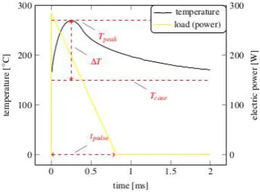
When conducting an accelerated life test for semiconductor devices in a lab, the stress is produced on the test system by a sequence of electric pulses. Their intensity depends on the setting of the electric input parameters, such as 𝑉 (voltage), 𝐼 (current) and 𝑡𝑝𝑢𝑙𝑠𝑒 (pulse length). The time period in which one pulse is performed is called a test cycle - as test cycles are the time unit in accelerated life testing, the total lifetime is measured in cycles to failure (𝐶𝑇𝐹).
The electric load of the pulses evokes a heat-up of the material, which is the main source of degradation. Especially the peak temperature 𝑇𝑝𝑒𝑎𝑘 (the maximum temperature which is reached in the device) and the temperature rise Δ𝑇 (difference between the case temperature 𝑇𝑐𝑎𝑠𝑒 and 𝑇𝑝𝑒𝑎𝑘 ) are important. The relation between these parameters is shown in Fig. 1
[3].
To transfer the process of increasing device degradation over time into mathematics, it is described by a non-negative, monotonically increasing function.
The failure of the device occurs when this so-called degradation function [4] reaches a critical threshold (usually a normalized scale with threshold 1 is used). A comprehensive interpretation of such a degradation function is to regard it as the "portion (or percentage) of consumed lifetime up to the current point in time".
Vol. 3 Issue 2, February - 2017 Unfortunately real use-conditions of the devices are
not constant - instead, they are exposed to stresses with varying intensities over time. For devices in the automotive industry, this is caused e.g. by temperature differences, dependent on seasonal or day/night changes, or by occasional failure events like short circuits. Together, these time periods are considered as a specific stress profile, also called a mission profile. It is therefore necessary to build a lifetime model for a sequence of stress intensities applied to one device within a lifetime study.
In order to describe the concept of mission profiles in a statistical way, a medical approach on so-called crossover studies (studies where multiple treatments are applied to one single test-object in a temporal order) is used [5]. As this medical model does not totally fit the given applications, several modifications of this approach are necessary to derive a model which is applicable to lifetime testing.
II. THE MODEL FOR CROSSOVER STUDIES
A. Basic crossover designs from medicine
As presented in [5], the classical model for crossover studies in a medical context is given by
𝑦𝑖,𝑗= 𝜇 + 𝛼𝑖+ 𝛽𝑗+ 𝜏𝑑(𝑖,𝑗)+ 𝜌𝑑(𝑖−1,𝑗)+ 𝜖𝑖,𝑗. (1) In this formula, the index 𝑖 ∈ {1, … , 𝑝 } refers to the period, 𝑗 ∈ {1, … , 𝑁 } refers to the subject. 𝜇 is the grand mean, 𝛼𝑖 denotes the effect of the 𝑖th period and 𝛽𝑗 denotes the effect of the 𝑗 th subject. 𝑑(𝑖, 𝑗) represents the treatment, which is applied to subject 𝑗 in period 𝑖. 𝜏𝑑(𝑖,𝑗) is the main effect of 𝑑(𝑖, 𝑗) and 𝜌𝑑(𝑖−1,𝑗) is the carry-over effect of treatment 𝑑(𝑖 − 1, 𝑗), i.e. the residual effect of the previous period, which influences the following treatment.
In a medical context carry-over effects are unwanted side-effects that have to be considered although they are not of any interest. Unfortunately carry-over effects can only be avoided by choosing a long washout-period, i.e. a long time gap between two treatments. This is not possible in medicine for reasons of ethics - leaving an ill patient without any treatment would not be justified for the purpose of a medical investigation. Therefore the modeling of the carry-over effect cannot be avoided.
B. Modifications of the model
The carry-over effect is the main factor of interest when adopting the model to mission profile tests for semiconductor devices. From previous work [6], lifetime models including parameter estimates for accelerated life testing under constant stress conditions are available and can be used to build a model for a sequence of different treatments, based on the semantic idea of the crossover study.
Intuitively it is probable that the carry-over effect of the 𝑖th period depends on the main effects of the previous treatments. Therefore it is assumed that the
carry-over effect is proportional to the main effect of the previous treatment, i.e.
𝜌𝑑(𝑖−1,𝑗)∝ 𝜏𝑑(𝑖−1,𝑗).
Higher-order dependencies of the carry-over effect (i.e. dependencies on 𝜏𝑑(𝑖−2,𝑗), 𝜏𝑑(𝑖−3,𝑗),…) are not considered at this point as the number of periods 𝑝 is restricted to 2 to reduce complexity. Further the additive terms for 𝛼𝑖 and 𝛽𝑗 are considered as being negligible for the purpose of semiconductor life testing, because the period itself has no additive influence on the response and all devices are assumed to be produced without any pre-damage.
A fundamental question that arises is how to define the response 𝑦𝑖,𝑗 in the experiment. As the survival time of the device under test is modeled, a proper choice would be to assign a lifetime to the response. Unfortunately the lifetime for semiconductor mission profile testing cannot be measured in each period, but only at the end of the test. It is therefore necessary to set 𝑦𝑗: = 𝑦2,𝑗 (which analogously requires to set 𝜖𝑗: = 𝜖2,𝑗). The resulting model is given by
𝑦𝑗= 𝜇 + 𝜏𝑑(2,𝑗)+ 𝛾𝜏𝑑(1,𝑗)+ 𝜖𝑗. (2) In this modified version of (1), 𝑗 ranges from 1 to 𝑁, but only one response per experimental object is observable. Nevertheless the semantic idea of the model is to add one parameter describing the second stress (last period) and one referring to the history the device experienced (carry-over effect).
In order to finally use this modified model for mission profile testing, it is necessary to define the responses 𝑦𝑗 and the effects 𝜏𝑑(1,𝑗) and 𝜏𝑑(2,𝑗) in terms of the experimental setup. For this purpose another method, the so-called Miner's rule, has to be introduced.
C. Mission profile testing
For this investigation, it is assumed that a device is consecutively exposed to two distinct stress conditions - stress period 1 and stress period 2. In the following, the number of cycles the object spends within each period are denoted by 𝑡1 and 𝑡2, respectively. Further 𝐶𝑇𝐹𝑖, 𝑖 ∈ {1,2}, are defined as the cycles to failure, if the stress condition of the 𝑖th period would have been applied constantly until the device fails.
An approach for dealing with this situation of two distinct stress periods in a deterministic model is given by the Miner's rule [7]. The Miner's rule claims that, regarding one device, summing over the portions of period duration 𝑡𝑖 divided by the full lifetime 𝐶𝑇𝐹𝑖 under the given stress level equals to 1, i.e. for two periods
∑ 𝑡𝑖 𝐶𝑇𝐹𝑖 2
𝑖=1 = 1. (3)
order to deal with the suggested model without being able to observe 𝐶𝑇𝐹𝑖, it is regarded as a random variable. This random variable is modeled by a separate regression model for constant stress conditions, e.g. see [1], called the single-treatment lifetime model for the 𝑖th stress period.
Using these single-treatment lifetime models, estimators 𝐶𝑇𝐹̂𝑖 for the expected values 𝐸(𝐶𝑇𝐹𝑖) can be derived and inserted into the Miner's rule, which then changes to
∑ 𝑡𝑖 𝐶𝑇𝐹𝑖̂ 2
𝑖=1 = 1.
Returning to the modified model for crossover studies presented in (2), Miner's rule implies the necessary relations in order to define 𝑦𝑗 and 𝜏𝑑(𝑖,𝑗), 𝑖 ∈ {1,2}. First we choose that the response 𝑦𝑗= 𝑡2, i.e. the survival time of the jth device in the second (and therefore last) period. Rearranging the Miner's rule to 𝑡2 leads to
t2= CTF2̂ −CTF̂2 CTF̂1⋅ t1.
Taking this formula as a basis, the single-treatment effects 𝜏𝑑(𝑖,𝑗), 𝑖 ∈ {1,2}, from the derived model in (2) are chosen as given below:
𝜏𝑑(𝑖,𝑗)= 𝐶𝑇𝐹̂2,𝑗 𝐶𝑇𝐹̂1,𝑗⋅ 𝑡1,𝑗
𝜏𝑑(2,𝑗)= 𝐶𝑇𝐹̂2,𝑗
Inserting these parameters into the model in (2), an additional model parameter 𝛾2 for the first term is added to ensure more flexibility. This results in the following linear model for mission profile testing:
𝑡2,𝑗= 𝜇 + 𝛾2𝐶𝑇𝐹2,𝑗+ 𝛾1𝐶𝑇𝐹2,𝑗 ̂
𝐶𝑇𝐹̂1,𝑗𝑡1,𝑗+ 𝜖𝑗.
Setting 𝜇 = 0, 𝛾2= 1 and 𝛾1= (−1), this model equals to the Miner's rule presented in (3), for each device 𝑗 if the error 𝜖𝑗 is 0.
III. OPTIMAL DOE FOR MISSION PROFILE TESTING Apart from building an appropriate model, it is necessary to select an appropriate DoE approach for it. A fundamental choice is whether classical DoE (full or fractional factorial designs) or optimal DoE shall be used.
In this paper optimal DoE is chosen, because this offers significant advantages. Some of these advantages for the given problem, according to [8], are:
Optimal DoE can cover restrictions on the design space, which is necessary as either the test system might not be able to apply all combinations of electrical parameters, or they are not feasible for a given product. The number of experimental units that are
available can be specified when using optimal DoE.
Prior knowledge about the model can be included when selecting an optimal design (Bayesian optimal DoE).
The most relevant drawback of optimal DoE is that the complexity of the concerned methods is higher - leading to higher effort for the DoE.
A. D-optimality criterion
When applying optimal DoE an important choice is to select an appropriate design criterion Ψ, which is used to optimize the design over the design space Ξ. In the given case, D-optimality (i.e. minimal volume of the confidence ellipsoid of the estimator for the model parameters) is used. For this purpose, the design information matrix is defined in the following way:
𝐼 = 𝑋′𝑋.
𝑋 denotes the design matrix containing all selected design points. The design criterion Ψ is defined as the determinant of 𝐼, i.e. Ψ(𝐷) = |𝐼|, 𝐷 ∈ ΞN. An optimal design 𝐷𝑜𝑝𝑡 including 𝑁 design points is found if
𝐷𝑜𝑝𝑡 = argmax𝐷∈Ξ𝑁Ψ(𝐷).
The D-optimality criterion leads to a unique optimal design information matrix 𝐼 , but several different optimal designs 𝐷𝑜𝑝𝑡 share the same 𝐼. Therefore a secondary design criterion Ψ2 is needed to improve the selection of an optimal design. As design points can be repeated in optimal designs, we define 𝑤 as the vector of weights, indicating how often each design points is chosen, and set 𝑋 as the matrix of the 𝑞 distinct design points 𝑥1, … , xq of the design. With this the design information matrix can be re-written as:
𝐼 = ∑ 𝑤𝑞𝑖 𝑖𝑥𝑖𝑥𝑖′. (4) Under all D-optimal designs for semiconductor lifetime testing, a design with a high number of points and a balanced weight vector is preferred - i.e. the secondary optimality criterion is defined by:
Ψ2(𝐷) = ‖𝑤𝐷‖2 𝐷… 𝐷−𝑜𝑝𝑡𝑖𝑚𝑎𝑙→ 𝑚𝑖𝑛
Although both criteria Ψ and Ψ2 do not ensure uniqueness of the resulting optimal design, each resulting design fulfills all requirements for an efficient lifetime study and therefore no further selection will be made.
B. Bayesian optimal DoE
Vol. 3 Issue 2, February - 2017 were available and hence it can reduce the testing
effort.
For Bayesian DoE methods for linear regression models, only the prior covariance matrix Σ is of interest. The design information matrix is extended by the prior to
𝐼𝐵= 𝐼 + Σ−1.
The optimality criterion for the Bayesian approach is called 𝐷𝐵-optimality and can be calculated in the same way as without prior knowledge, but using the Bayesian design information matrix 𝐼𝐵. Therefore, the 𝐷𝐵-optimality criterion Ψ𝐵 is defined as Ψ𝐵(𝐷) = |𝐼𝐵|, the optimal design fulfills
𝐷𝑜𝑝𝑡 = arg max𝐷∈Ξ𝑁Ψ𝐵(𝐷). (5) Since prior information increases the certainty about the parameter estimates, the volume of the parameter confidence ellipsoid is reduced, leading to a larger value of the information criterion. Consequently, the following relation holds:
Ψ𝐵(𝐷) > Ψ(𝐷) ∀𝐷 ∈ Ξ𝑁.
C. Exchange algorithm
In general it is not trivial to find a design 𝐷𝑜𝑝𝑡, which is optimal with respect to the mentioned optimality conditions, therefore an algorithm for the optimization is needed. A popular class of algorithms for optimal DoE, which are applicable to various different optimality criteria, is the class of exchange algorithms based on the famous Fedorov algorithm [10]. Many modifications of the latter are available, in the given context the version by Cook and Nachtsheim from [11] is used.
Starting with an initial design 𝐷0 (which is assumed to be random in this work), each point 𝑥𝑖 in the design is replaced by the point 𝑥𝑖∗ from the design space Ξ, which maximizes the value of the optimality criterion Ψ given that all other points 𝑥𝑗, 𝑗 ≠ 𝑖, are fixed. Applying this procedure sequentially on each design point in 𝐷 until no further improvement is possible leads to an optimal design 𝐷𝑜𝑝𝑡.
The exchange algorithm is implemented in several packages in different programming languages. For the practical example in Section IV, a package in the programming language R was implemented.
IV. PRACTICAL EXAMPLE
In order to show how the described model for mission profile testing is applied in practice, the following example is used: two specific single-treatment lifetime models are chosen according to results from previous research. The idea behind is to simulate a normal load condition (use-case), followed by an overload condition.
A. The model setup
The first treatment (treatment 1) is used to simulate a use-case, the other is used for testing under overload conditions (treatment 2). Single-treatment models for both situations, i.e. lifetime models for constant load over the whole testing time, are presented in [1]. The time of the first treatment is set as an additional input parameter 𝑡1,𝑗.
The use-case treatment is simulated using the following generalized linear model
𝑙𝑜𝑔(𝐶𝑇𝐹1) = 𝑙𝑜𝑔(𝐴1) + 𝛼 𝑙𝑜𝑔(𝑡𝑝𝑢𝑙𝑠𝑒) + 𝛽1 𝑙𝑜𝑔(Δ𝑇1) +𝑘 𝑇Δ𝐻
𝑝𝑒𝑎𝑘 + 𝜖1. (6)
In this model 𝑘 is the Boltzmann constant, 𝑙𝑜𝑔(𝐴1), 𝛼, 𝛽1 and Δ𝐻 are the model parameters and 𝑡𝑝𝑢𝑙𝑠𝑒, Δ𝑇1 and 𝑇𝑝𝑒𝑎𝑘 are the input parameters of the model as introduced in Fig. 1.
In a similar, reduced way, the second treatment is described by
𝑙𝑜𝑔(𝐶𝑇𝐹2) = 𝑙𝑜𝑔(𝐴2) + 𝛽2 𝑙𝑜𝑔(Δ𝑇2) + 𝜖2. (7) Compared to the model given in (6), the set of input parameters for this model reduces to one single parameter Δ𝑇2, due to the setup of the applied test pulse.
The intervals for the ranges of the input parameters for both models are presented in TABLE 1.
To apply one single treatment over the whole lifetime of a device, the model parameters log(A1), log(A2), α, etc. of each of these two models in (6) and (7) are available from previous works [6].
The design space Ξ of the mission profile test contains the parameters of both treatments and the number of cycles of the first treatment t1, i.e. each d ∈ Ξ is 5-dimensional:
d =
( t1 ΔT1 Tpeak tpulse ΔT2 )
.
TABLE 1:RANGES FOR INPUT PARAMETERS OF THE SINGLE-TREATMENT LIFETIME MODELS
Parameter Treatment 1 Treatment 2
Δ𝑇 [150,250] [250,350]
𝑇𝑝𝑒𝑎𝑘 [300,350] −
𝑡𝑝𝑢𝑙𝑠𝑒 [0.2,3.5] −
For a given set of input parameters Δ𝑇1,𝑗 , Δ𝑇2,𝑗, 𝑇𝑝𝑒𝑎𝑘, …, the estimators for 𝐶𝑇𝐹̂1 and 𝐶𝑇𝐹2̂ can be calculated by using the estimators for the model parameters of both single-treatment lifetime models (6) and (7), available from [6]. The design matrix 𝑋 for the model for mission profile testing can be obtained, according to (4), by
𝑥𝑗 = ( 1 𝐶𝑇𝐹̂2,𝑗 𝐶𝑇𝐹2,𝑗̂ 𝐶𝑇𝐹1,𝑗̂ 𝑡1,𝑗
) .
With this, the information matrix 𝐼 = 𝑋′𝑋 can be calculated, which is necessary to apply an optimality criterion for DoE.
B. Prior information for Bayesian approach
To apply the Bayesian approach on optimal DoE it is necessary to specify a prior distribution. For this example, the prior is defined by heuristic means.
A special case of the model is the Miner's rule - in case that the Miner's rule fits the data exactly, the values for the model parameters are 𝜇 = 0, 𝛾2= 1 and 𝛾1= (−1). The selection of this set of parameters is therefore considered as the prior mean. The prior variance of the mean 𝜇 is assumed to be high as no information about this parameter is available - the a-priori variance is chosen as 𝜎1,12 = 100. According to observations from foregoing experiments, 𝛾2 and 𝛾1 are assumed to be in a range of ±1 around their mean values with a probability of 0.9, i.e. 𝜎2,22 = 𝜎3,32 ≈ 0.37. This choice leads to the issue that the value 0 is possible for both parameters according to the prior, nevertheless it is not realistic regarding the deduction of the model, but specifying a more informative prior is not justified. Further, independence is assumed for the parameters, which leads to the prior covariance matrix
Σ = (1000 0.370 00 0 0 0.37) .
For the calculation of the information criterion in the context of the Bayesian approach, the 𝐷𝐵-optimality criterion needs to be applied: Due to the incorporation of prior information, in general higher values of the design criterion Ψ𝐵, defined in (5), compared to Ψ are returned even for randomized designs.
More accurate prior knowledge may be available in the future, after completing further physical investigations about the damaging process.
C. Design optimization for mission profile testing
For the concrete case in this example, an initial design 𝐷𝑖𝑛𝑖𝑡 with 16 design points is sampled and then optimized (with and without a Bayesian approach). The resulting D-optimal design 𝐷𝑜𝑝𝑡 (without prior) and the 𝐷𝐵-optimal design 𝐷𝑜𝑝𝑡𝐵 are created by applying the Fedorov exchanged algorithm explained in Subsection III.C.
Apart from 𝐷𝑖𝑛𝑖𝑡, 𝐷𝑜𝑝𝑡 and 𝐷𝑜𝑝𝑡𝐵 , an additional design is introduced for reasons of comparability: a full factorial design from classical DoE is approximated. The approximation is needed because the described restrictions of the design space do not allow the use of an exact full factorial design.
By sampling random values from the given input ranges (see TABLE 1), points on the design space are
simulated via the calculation of their single-treatment expected lifetime. Analog to the classical DoE theory [12], the minimum and maximum lifetimes are used for the approximated classical DoE. This design is denoted by 𝐷𝑐𝑙𝑎𝑠𝑠𝑖𝑐 and shall represent a more heuristic design selection procedure compared to the other approaches.
To compare these four designs, the first characteristic number is given by the value of the design functional Ψ. As the absolute value of Ψ is dimensionless, the increase compared to Ψ(𝐷𝑖𝑛𝑖𝑡), which is related to the gained information, is calculated.
Unfortunately real test results are not available yet, but for a detailed comparison of the increase in information by optimal DoE, a set of simulated data is used to sample responses for the mission profile test with predefined parameters. With this simulated data set, the model parameters 𝜇, 𝛾2 and 𝛾1 are estimated. The standard error of the estimated parameters is then inversely linked to the information given by the optimality criterion, meaning that the lower the error, the higher the level of information.
V. RESULTS
Based on a randomly sampled initial design 𝐷𝑖𝑛𝑖𝑡 containing 16 distinct design points (without replication), the exchange algorithm returns an optimized design 𝐷𝑜𝑝𝑡 with 5 different design points. The associated weights vector 𝑤 = (5,4,3,3,1)𝑇, which means that the single points are repeated one to five times each. Graphically, they are widely distributed over the design space.
Vol. 3 Issue 2, February - 2017 In the classic design 𝐷𝑐𝑙𝑎𝑠𝑠𝑖𝑐, the number of distinct
design points is predefined by selecting the maximum and the minimum on each of the two coordinate axes, resulting in 4 data points. The weights are set to 𝑤 = (4,4,4,4)𝑇.
The resulting values of the design criterion Ψ applied to the designs and their relative increase compared to Ψ(𝐷𝑖𝑛𝑖𝑡) are shown in TABLE 2. It is important to consider that the value for 𝐷𝑜𝑝𝑡𝐵 is calculated using the design criterion Ψ𝐵 including the prior information, which leads to a higher absolute value, which is not directly comparable to the absolute value of the other designs. The relative raise for this design is lower than for the other designs as the prior information is already taken into account for the initial design 𝐷𝑖𝑛𝑖𝑡.
After comparing the values of the design criterion, the responses of the mission profile test are simulated for each design points of 𝐷𝑖𝑛𝑖𝑡, 𝐷𝑐𝑙𝑎𝑠𝑠𝑖𝑐, 𝐷𝑜𝑝𝑡 and 𝐷𝑜𝑝𝑡𝐵 by using predefined model parameters (𝜇 = 100, 𝛾2= 0.8, 𝛾1= −1.4) and randomly generated errors with a 𝑁(0,25) distribution. Using this data, the model parameters and their standard errors are estimated by the least squares method and presented in TABLE 3. For the Bayesian design, the prior information is considered in the least squares estimation.
For the comparison of the designs, the standard error is a more significant quality criterion than the point estimators, because if the design points are spread over the whole design space, slight variations do not affect the point estimator significantly (see:
TABLE 3). Instead the standard error reflects the quality
of information given in the data. As a result of the investigation, one can see that the standard errors for the model for mission profile testing parameter estimates decrease from 𝐷𝑖𝑛𝑖𝑡 to 𝐷𝑐𝑙𝑎𝑠𝑠𝑖𝑐 by factors up to 2. Comparing 𝐷𝑐𝑙𝑎𝑠𝑠𝑖𝑐 and 𝐷𝑜𝑝𝑡 , a further improvement by nearly the same factor is achieved. The Bayesian design 𝐷𝑜𝑝𝑡𝐵 leads to the smallest error of all designs, meaning that this design will provide data with the highest level of information.
Finally, modeling mission profiles using the suggested model is possible and applicable for the described problem. Optimal DoE significantly improves the information gained out of a study and can even be enriched with the use of a-priori knowledge.
TABLE 2:COMPARISON OF DESIGN CRITERION VALUE Ψ OF THE DESIGNS
Design Absolute value Relative raise
𝐷𝑖𝑛𝑖𝑡 60.5 −
𝐷𝑐𝑙𝑎𝑠𝑠𝑖𝑐 487.3 8.05
𝐷𝑜𝑝𝑡 1600 26.44
𝐷𝑜𝑝𝑡𝐵 2697 4.79
TABLE 3:ESTIMATED MODEL PARAMETERS AND STANDARD ERRORS FOR
THE FOUR COMPARED DESIGNS
𝐃𝐢𝐧𝐢𝐭 𝐃𝐜𝐥𝐚𝐬𝐬𝐢𝐜 𝐃𝐨𝐩𝐭 𝐃𝐨𝐩𝐭𝐁
Estimates
𝜇̂ 104.73 93.16 97.71 95.69
𝛾2̂ 0.80 0.80 0.80 0.80
𝛾̂1 −1.40 −1.40 −1.40 −1.40
Standard Errors
𝜇̂ 2.0 ∗ 101 2.0 ∗ 101 2.0 ∗ 101 2.0 ∗ 101
𝛾2̂ 2.1 ∗ 10−3 2.1 ∗ 10−3 2.1 ∗ 10−3 2.1 ∗ 10−3
𝛾̂1 4.6 ∗ 10−3 4.6 ∗ 10−3 4.6 ∗ 10−3 4.6 ∗ 10−3
VI. CONCLUSION
In summary, the task was to derive a statistical model for the lifetime of a semiconductor device under a mission profiles in order to efficiently apply accelerated life testing. An approach from medicine, the so-called crossover study model was introduced and modified for this purpose. After several transformations and considerations, the resulting model is also a generalization of the Miner's rule, which describes the cumulative effect of different stress intensities.
To optimize the gain of information in the study at a limited number of performed tests, optimal DoE is applied. Therefore, the D-optimality criterion is used, combined with an approach to select balanced designs, realized by a secondary optimality criterion. Then a modified version of the Fedorov exchange algorithm is used in order to generate an optimal design out of a randomized initial design. Additionally a-priori information can be introduced by using a Bayesian optimal DoE approach, which is also compatible with the employed algorithm.
In a practical example with two specific single-treatment lifetime models and 16 design points, different designs were analyzed and compared. In the end, the optimized design for crossover studies provided a significantly higher gain of information compared to the randomized initial design and to a classical full-factorial design.
Several generalizations of the suggested model would be possible. One example would be to increase the number of periods, which was set to 2 in this study. This is possible using the suggested derivation of the model. Nevertheless the case of devices failing before the last period have to be taken into account in this case.
mission profile test for semiconductor devices applying the proposed model and procedure.
ACKNOWLEDGEMENT
At this point we would like to thank Anja Zernig (KAI) for testing the implemented software during the preparation of this paper, supporting the presented results.
This work was jointly funded by the Austrian Research Promotion Agency (FFG, Project No. 846579) and the Carinthian Economic Promotion Fund (KWF, contract KWF-1521/26876/38867).
REFERENCES
[1] O. Bluder, "Prediction of Smart Power Device Lifetime based on Bayesian Modeling," 2011. [2] K. Plankensteiner, "Application of Bayesian
Models to Predict Smart Power Switch Life Time," 2011.
[3] S. Schrunner, "Optimal Experimental Design for Crossover Semiconductor Lifetime Studies," 2016.
[4] S. Schrunner, "Bestimmung der First-Passage-Time Verteilung von Degradation-Path-Modellen," 2014.
[5] M. Bose and A. Dey, "Crossover Designs," in Handbook of Design and Analysis of
Experiments, A. Dean and others, Eds., CRC Press, 2015.
[6] K. Plankensteiner, "Application of Bayesian Networks and Stochastic Models to Predict Smart Power Switch Lifetime," 2015.
[7] M. A. Miner, "Cumulative Damage in Fatigue," Journal of Applied Mechanics, 1945.
[8] F. Triefenbach, "Design of experiments: The D-optimal approach and its implementation as a computer algorithm," 2008.
[9] J. Pilz, Bayesian Estimation and Experimental Design in Linear Regression Models, John Wiley and Sons, 1991.
[10] V. V. Fedorov, Theory of Optimal Experiments, Academic press, 1972.
[11] A. Mandal, W. K. Wong and Y. Yu, "Algorithmic Searches for Optimal Designs," in Handbook of Design and Analysis of Experiments, A. Dean and others, Eds., CRC Press, 2015.
[12] M. D. Morris, Design of Experiments - An