On the Hardness of Learning With Errors with Binary Secrets

www.theoryofcomputing.org

On the Hardness of Learning With Errors

with Binary Secrets

Daniele Micciancio

Received September 17, 2017; Revised October 13, 2018; Published November 30, 2018

Abstract: We give a simple proof that the decisional Learning With Errors (LWE) problem with binary secrets (and an arbitrary polynomial number of samples) is at least as hard as the standard LWE problem (with unrestricted, uniformly random secrets, and a bounded, quasi-linear number of samples). This proves that the binary-secret LWE distribution is pseudorandom, under standard worst-case complexity assumptions on lattice problems. Our results are similar to those proved by Brakerski, Langlois, Peikert, Regev and Stehlé (STOC 2013), but provide a shorter, more direct proof, and a small improvement in the noise growth of the reduction.

1

Introduction

The Learning With Errors (LWE) problem [21,22] plays a central role in lattice cryptography, its secure instantiation, and its most advanced applications. The usefulness of LWE in cryptography is due in large part to its pseudorandomness properties, captured by the standard decisional LWE problem defined as follows. An LWE instance is described by a matrixA∈Zm×nq (chosen uniformly at random) and a vector

∗_{Research supported in part by the Defense Advanced Research Project Agency (DARPA) and the U.S. Army Research}

Office under the SafeWare program, and the National Science Foundation (NSF) under grant CNS-1528068. Any opinions, findings, and conclusions or recommendations expressed in this material are those of the author(s) and do not necessarily reflect reflect the views, position or policy of the Government.

ACM Classification:F.2.2, F.1.3

AMS Classification:68Q17, 52C07, 11H06

b∈_Zm

q which may be chosen either uniformly at random, or asb=As+e (modq), wheres∈Znqis a

random secret ande∈_Zm_{is a “small” error vector, typically chosen with independent discrete Gaussian}

entries of standard deviationσ≈

√

n. The (Decisional) LWE problem asks to distinguish between these two cases.

Several variants of LWE exist in the literature, depending on howsandeare chosen, all motivated by specific cryptographic applications. In the most standard formulation of LWE, the secrets∈_Zn

qis

chosen uniformly at random. But this is often undesirable in many cryptographic applications, e. g., those making use of modulus-switching techniques, where large secrets result in substantial ciphertext quality degradation. Ideally, it would be best to chooses∈ {0,1}n_{as a vector with binary entries, as used for}

example in many Fully Homomorphic Encryption schemes (e. g., see [9,8]). This binary-secret LWE also plays a fundamental role in theoretical studies, like the proof that LWE is leakage resilient [11], and the proof that LWE with polynomial modulusqis at least as hard as worst-case lattice problems under classical (i. e., non-quantum) reductions [6].

This last work [6] is the best currently known hardness result for binary-secret LWE, and gives a reduction from (standard) LWE with arbitrary secret inZnq, to LWE with secret in{0,1}nlogq, i. e., the

secret can be restricted to binary vectors at the cost of increasing the dimension1fromntonlogq. This reduction is a major part of the main result of [6] on the classical hardness of LWE, and takes a good half of that paper, going through a careful hybrid argument involving some technical (“first-is-errorless” and “extended-LWE”) problem variants.

In this paper we present a direct and substantially shorter proof of this important result. In fact, while the proof of this result given in [6] is over 7 pages long, spanning multiple subsections, and involving a number of intermediate problems, our proof has a more direct structure and it is much shorter. A key insight leading to our simpler proof is the formulation of the binary LWE problem (denotedLWE±) using secrets in{±1}n_{, rather than{0,1}}n_{. This is easily seen (for odd}2_{modulusq) to be equivalent to} the more common{0,1}formulation via the affine transformations7→(2s−1), but has the technical advantage that all secrets have exactly the same Euclidean length, simplifying the application of discrete Gaussian convolution theorems. Given the equivalence between the two problems, we will keep referring toLWE±informally as the binary LWE problem. Other than presenting a simpler and shorter proof, we do not claim any new results over previous work: our results, and the range of parameters for which we reduceLWEtoLWE±, are essentially the same as in [6, Theorem 4.1], except possibly for reducing some constants, e. g., in our reduction the error grows by a factor 2√n+1, while in [6, Theorem 4.1] it grows by√10n.

Given the important role played by binary LWE in many cryptographic applications, we hope that our simplified treatment will make the theoretical hardness of this problem more easily accessible, and stimulate further research.

Related work. The LWE problem with small secret was first formally considered by Applebaum, Cash, Peikert and Sahai in [3], who proved that, without loss of generality, one may assume that the secret

1_{As remarked in [6], this increase seems unavoidable, as it preserves the bit-length of the secret.}

2_{Hardness results for binary LWE withevenmodulusqare easily obtained by modulus switching, i. e., scaling and (randomly)}

rounding each entryx∈ZqofAorbbx·((q−1)/q)e$∈Zq−1. This increases the error roughly by an additive termO(ksk),

follows the same distribution as the LWE errors. This allows the secret coordinates to be as small as√n, but not as small as{0,1}. For a list of applications using LWE with small secrets see [1].

Reducing LWE to have a binary secret was first considered by Goldwasser, Kalai, Peikert and Vaikuntanathan in [11], motivated by questions in leakage-resilient cryptography, where the problem is proved hard using “noise-flooding” techniques. A stronger reduction is given by Brakerski, Langlois, Peikert, Regev and Stehlé in [6], in the context of proving classical hardness results for LWE.

A different (and much harder) problem is that of proving that LWE is computationally hard when the

error(and not just the secret) follows the binary distribution [17,7]. In fact, LWE with small errors can be efficiently solved when sufficiently many samples are available [4,2,13]. In this paper, we do not study LWE with binary errors.

Attacks against LWE with binary secret (and Gaussian errors) are considered in [1,5]. Theoretically, the secret can be assumed binary by increasing the LWE dimension tonlogq[6], but experimental results in [5] suggest that, heuristically, increasing the secret dimension by a log lognfactor may already be enough to counter the best known cryptanalytic attacks for common parameter settings.

Paper organization. In Section 2we introduce the notation used in this paper, provide a formal definition of the LWE problem, and present some background results, including a simple lemma on the projection of discrete Gaussians (Lemma 2.6), and the construction of a gadget matrix needed in our main reduction (Lemma 2.7). The proof that LWE with binary secrets is pseudorandom is given inSection 3.

Section 4concludes with a discussion of open problems.

2

Preliminaries

We use bold lowercase lettersafor vectors, and bold uppercaseAfor matrices. Probability distributions are denoted using calligraphic lettersA. We write vectors as columnsv∈_Zn₌

Zn×1. The transpose of a vector or matrixAis denotedAt_{. We write[A}

1, . . . ,An]for the horizontal concatenation of matrices

Ai∈Zk×mi_{, and use transpose notation[A}

1, . . . ,An]t for the vertical concatenation ofAt1, . . . ,Atn. Let e1, . . . ,enbe the standard basis ofZn,I= [e1, . . . ,en]then×nidentity matrix, andu=∑ieithe all-ones

vector. The Euclidean norm of a vector is

kxk=

r

∑

i x2_i,

and the max norm iskxk_∞=maxi|xi|.

For any vectorz= (z1, . . . ,zn)∈Zn, we writediag(z) = [z1·e1, . . . ,zn·en]for the diagonal matrix with the entries ofzalong the diagonal. So, for example,diag(u) =I. For any integer matrixQ∈Zn×m and for any positive integerk≤m, we writeQ[k]for the matrix consisting of the firstkcolumns ofQ,

andQ_]k[ for the matrix obtained by removing the firstk columns fromQ. So,Q= [Q[k],Q]k[]where

Q[k]∈Zn×k andQ]k[∈Zn×(m−k).

For any integer matrixQ∈_Zk×m, we write ker(Q) ={x∈_Zm_{:Qx=0}for the kernel ofQ:}

Zm→Zk as an integer linear map. We say that a matrixQ∈_Zk×m_{isprimitiveifQ}

2.1 Probabilities and asymptotics

We use standard asymptotic notation,O(·),Ω(·)andω(·), and all asymptotics refer to a (possibly implicit)

integer variablen. For example, we may writenO(1)for an arbitrary polynomially bounded function ofn, andn−ω(1)_{for a negligible function. Other parameters defining the size of a problem instance are always}

assumed to be polynomial inn. So, ifA∈_Zk×mis a matrix with integer entries, the number of rows

k=nO(1), the number of columnsm=nO(1), and the bitsize maxi,jlog|ai,j|=nO(1)of the matrix entries

are all assumed to be (at most) polynomial inn.

A probability ensemble is a sequence An of probability distributions over sets An, for n∈N= {1,2, . . .}. We always assume that all elements ofAn⊆ {0,1}`(n)_{can be represented by strings of some}

fixed length`(n). We writex←Afor the operation of sampling an elementxaccording to distributionA, and Pr{x←A}for the probability ofxunderA. The uniform distribution over a setAis denotedU(A).

Thestatistical distancebetween two distributionsA,A0over a setAis

∆(A,A0) =1

2_x∈A

∑

0_}| .

Two distribution ensemblesAn,A0n arestatistically close(writtenAn≈A0n) if the statistical distance

∆(An,A0n) =n−ω(1)is negligible. Two ensemblesAn,A0narecomputationally indistinguishableif for any

efficient (probabilistic polynomial-time computable) predicateP,P(An)≈P(A0n). The gap

∆(P(An),P(A0n)) =|Pr{P(An)} −Pr{P(A0n)}|

is called theadvantageofPin distinguishing between the two distributions. An ensembleAnover sets Anispseudorandomif it is computationally indistinguishable from the uniform distributionsU(An). If

An≈U(An)are statistically close, then we say thatAnis almost uniform or statistically pseudorandom.

We typically leave the parameternimplicit, and talk about individual distributionsAover a single setA, but all asymptotic statements should be interpreted as referring to ensemblesAnparameterized

by an integernin some obvious way. For example, we may say that a distributionAover a setAis pseudorandom if no efficient algorithm can distinguishAfromU(A)with better than negligible advantage. More precisely, an efficiently sampleable ensemble{An}n>0over the sets{An}n>0is pseudorandom if any predicatePcomputable in probabilistic polynomial timenO(1)has at most negligible advantage

|Pr{P(An)} −Pr{P(U(An))}| ≤n−ω(1)

in distinguishingAnfrom the uniform distributionU(An).

We writeZfor the set of integers, andZq=Z/(qZ)for the integers moduloq. We will need the following version of the leftover hash lemma, and a bound on the probability that a random vector is primitive moduloq.

Lemma 2.1(Leftover Hash Lemma, [12]). For any odd integer q, positive realε >0and integers k

and n≥log₂(qk/ε2), the distributionX={(A,Az):A←U(Zk×nq ),z←U({±1}n)}is within statistical distance∆(X,U)≤ε from the uniform distributionU=U(Zk×nq ×Zkq). In particular, if n≥klog2(q) +

Lemma 2.2(Primitive Vectors). For any positive integers q=2nO(1)and k=ω(logn), ifw∈_Zk

qis chosen uniformly at random, thengcd(w,q) =1except with negligible probability.

Proof. The probability that gcd(w,q)6=1 is at most

∑

p|q

p−k≤(logq)/2k≤nO(1)/nω(1)_=n−ω(1)

where the summation is over all prime factors ofq. We used the fact that all prime factors are at least

p≥2, and there are at most log₂qof them. Better bounds are possible, but this crude estimate is more than enough for the purposes of this paper.

2.2 Gaussian distributions

Letρ(x) =exp(−πx2)be the Gaussian function with total massR

x∈_Rρ(x)dx=1, andρσ(x) =ρ(x/σ)

its scaling by a factorσ>0. For a setA, we writeρσ(A)as a shorthand for∑x∈Aρσ(A). The discrete

Gaussian distribution of parameterσ, denoted3Dσ, picks each integerx∈Zwith probability proportional toρσ(x), i. e., Pr{x←Dσ}=ρσ(x)/ρσ(Z). The product distribution Dkσ selects each x∈Z

k _with

probability proportional toρσ(x) =ρσ(kxk) =∏iρσ(xi). Ifxandyare orthogonal vectors (xty=0),

then by the Pythagorean theoremρσ(x+y) =ρσ(x)·ρσ(y).

A rank-ninteger lattice is the setΛ=BZn⊆Zd of all integer linear combinations ofn linearly independent vectorsB= [b1, . . . ,bn]inZd. The last successive minimum of a rank-nlatticeΛis the smallest positive realλnsuch thatΛcontainsnlinearly independent vectors of length at mostλn. Another

standard quantity associated to a lattice is the smoothing parameterηε(Λ), which is parameterized by a

positive realε>0. In this paper, all we need to know about the smoothing parameter are the following

two bounds.

Lemma 2.3(See [18, Lemma 4.1] and [10, Lemma 2.4]). For any latticeΛ,ε∈(0,1), and vectorcin

the linear span ofΛ, ifσ>ηε(Λ), thenρσ(Λ+c)∈[(1−ε)/(1+ε),1]·ρσ(Λ).

Lemma 2.4(Smoothing Parameter Bound, [18, Lemma 3.3]). For any rank-n latticeΛand positive real

ε>0, the smoothing parameter is at most

ηε(Λ)≤ r

ln(2n(1+1/ε))

π ·λn(Λ). (2.1)

In particular, for anyω(

√

logn)function there is a negligible functionε(n) =n−ω(1)such thatηε(Λ)≤

ω(

√

logn)·λn(Λ).

When the smoothing parameterη(Λ)is written without specifying the value ofε, it is assumed that ε=n−ω(1)is an arbitrary negligible function of the asymptotic variablen. For example, the smoothing

parameter of the integer lattice isη(Z)≤pln(2(1+1/ε)/π) =ω(

√

logn). We will also need the following convolution theorems for discrete Gaussians.

3_{In the literature,D}

σ is often used for the continuous Gaussian distribution over the real numbersR, while the discrete

Gaussian is denotedD_Z,σ. Since here we do not use continuous Gaussians, for brevity we useDσ to denote the discrete

Lemma 2.5(Convolution, [17, Theorem 3]). For any primitive vectorv∈_Zm_{and positive reals}

σi≥

√

2kvk_∞η(Z), if yi←Dσi for i=1, . . . ,m, then the sum y=∑ivi·yiis statistically close toDσ, where

σ=p∑i(viσi)2.

Lemma 2.6(Gaussian Projection). For any primitive matrixT∈Zk×m, positive realsα,σ >0, and

negligibleε =n−ω(1), ifT·Tt=α2·Iandη(ker(T))≤σ, thenT(Dm_σ)≈Dk_{α σ}.

Proof. Lety∈_Zk _{be an arbitrary integer vector, and letx∈}

Zmbe such thatTx=y. By linearity, any otherz∈_Zm_{maps toTz=yif and only ifz∈x+ker(T). So, by definition, the probability ofy=Tx}

underT(Dm_σ)is proportional toρσ(x+ker(T)). Letx1=Tty/α2∈Rmandx0=x−x1∈Rm, so that

x=x0+x1, andx0 is orthogonal to the rows ofT. It follows thatx1is orthogonal to x0 and ker(T). Therefore,ρσ(x+ker(T)) =ρσ(x1)·ρσ(x0+ker(T)). Sincex0 belongs to the linear span of ker(T), andσ≥η(ker(T)), byLemma 2.3the Gaussian massρσ(x0+ker(T))is essentially independent ofx0, up to a negligible relative error. So, up to this error, the probability ofyis proportional toρσ(x1). Finally, we observe thatkx1k2=ytTTty/α4=kyk2/α2, and therefore ρσ(x1) =ρσ(kyk/α) =ρα σ(y). This

proves thatT(Dm

σ)is statistically close to the discrete Gaussian distributionD

k

α σ.

2.3 A gadget matrix construction

Our main proof requires an integer matrix satisfying some special properties. In the following lemma, we state the required properties and give a simple construction. We recall that notationQ[n](resp.Q]n[)

stands for the matrix obtained by taking (resp. dropping) the firstncolumns of a matrixQ. In particular,

Q]1[is the matrixQwithout its first column.

Lemma 2.7. There is an efficiently computable matrixQ∈Zn×(2n+3)such thatQ[n]is invertible,utQ[n]=

et₁, the vectorvt =utQ]n[ has normkvk=2

√

n,kvk_∞=2, and the matrixT=Q]1[satisfiesT(D2σn+2)≈ Dn

2σ for allσ≥ω( √

logn).

Proof. Define the matrix

X=

n−1

∑

i=1

(ei+1−ei)·eti =



    

−1

1 . .. . .. −1

1



    

∈_Zn×(n−1)_.

The idea is to start with the square matrixQ¯ =Q¯[n] = [e1,X], which is unitriangular (i. e., triangular, with unit elements along the diagonal, and, therefore, invertible), and it satisfiesutQ¯ =et₁. We would like to useLemma 2.6 to analyze the distribution Q¯]1[(Dmσ) =X(D

m

σ). However, X is not primitive

and does not satisfy the propertyXXt ₌

α2Irequired byLemma 2.6because adjacent rows ofXhave

˜

Q= [Q,Y¯ ] = [e1,X,Y]with a block of(n−1)coordinates

Y=

n−1

∑

i=1

(ei+1+ei)·eti=

      1

1 . .. . .. 1

1      

∈_Zn×(n−1)

where adjacent rows have scalar product 1, and cancel out withX. This timeQ˜]1[= [X,Y]has pairwise

orthogonal rows, but the first and last rows have a different norm than the rest. So,[X,Y][X,Y]t _is

diagonal, but it is still not a scalar matrixα2I. We complete the construction by adding 4 more columns

to make each row ofQ]1[contain precisely 4 nonzero±1 entries. Our final construction is

Q= [e1,X,−en,Y,en,e1,e1]

where the position and sign of the new columns have been chosen to highlight the (square) unitriangular blocksX˜ = [X,−en],Y˜ = [Y,en]∈Zn×n. Notice thatY˜ =X˜ +2I, and therefore the two blocks commute, i. e.,X ˜˜Y=Y ˜˜X.

We already know thatQ[n]= [e1,X]is invertible,utQ[n]=et1, and it is immediate to verify that the vectorvt_=ut_Q

]n[satisfieskvk=2

√

nandkvk_∞=2. It remains to analyzeT(D2n+2

σ ), where

T=Q_]1[= [X,˜ Y,e˜ 1,e1].

This matrix is primitive because it starts with a unitriangular block, and it satisfiesTTt =4Iby con-struction. In order to applyLemma 2.6, and conclude thatT(D2n+2

σ )≈D2σ, we only need to bound the

smoothing parameter ofΛ=ker(T). This lattice is defined by a systemTx=0ofnlinearly independent equations in 2n+2 variables. So,Λis a rank-(n+2)lattice. Moreover, it contains(n+2)vectors of length at most 2 given by the columns of the matrix

V=     ˜

Y e1

−X˜ −e1

1 1

1 −1



  

∈_Z(2n+2)×(n+2).

The columns are linearly independent because the matrix

W=





I I

1 1

1 −1



∈Z(

n+2)×(2n+2)

satisfiesWV=2I. SoVhas rankn+2. This proves thatλn+2(Λ)≤2, and therefore, byLemma 2.4,

η(Λ)≤ω(

√

2.4 Computational problems and LWE

All computational problems considered in this paper are decision problems about pseudorandom distribu-tions. Specifically, for any distribution ensembleAnover setsAn, theAn-assumptionis the assumption

thatAnis pseudorandom, and theAn-problemis the computational problem of distinguishingAnfrom the

uniform distributionU(An)with non-negligible advantage. So, all problems will be implicitly specified simply by defining an appropriate set of distributionsAn.

A reduction between (the decision problems associated to) two distributionsAnandA0n over sets AnandA0_n(fromAntoA0n) is an efficient (probabilistic polynomial-time) algorithm that solves problem

An(i. e., distinguishesAnfrom the uniform distribution with non-negligible advantage) given access to

any oracle that solvesA0nwith (possibly different, but still) non-negligible advantage. In the simplest

settings (e. g., see Lemmas2.12and2.13) a reduction may be specified just by an efficient (probabilistic polynomial-time computable) functionϕ such thatϕ(An)≈A0nandϕ(U(An))≈U(A0n). Most of our

reductions are more complex, and make use of hybrid arguments (seeLemma 2.9) that require oracle calls on distributions other thanA0norU(A0n).

In this paper, it is convenient to consider a version of the Learning With Errors (LWE) problem where the secret is a matrixS, rather than a vector, defined as follows.

Definition 2.8. For any positive integers q,n,k,m and real σ, let LWE(q,n×k,m,σ) be the LWE

distribution with modulusq, number of samplesm, secret dimensionn×k, and error parameterσ, i. e.,

the distribution of

[A,AS+E]∈Zm×q (n+k)

obtained by pickingA←U(Zm×nq )andS←U(Zn×kq )uniformly at random, andE←Dm×kσ with discrete

Gaussian distribution.

When k=1, the secret is just a vector s∈_Zn

q, and this is the standard version of LWE, which

we writeLWE(q,n,m,σ) instead ofLWE(q,n×1,m,σ). Themrows of the LWE can be viewed as

random noisy labeled samples from a hard-to-learn linear function defined by the secretS. Worst-case to average-case reductions [21,19,6,20] support the conjecture that the LWE problem is hard for an arbitrary (polynomially bounded) number of samplesm=nO(1), and some reductions require this extra flexibility. (E. g., the LWE search-to-decision reduction in [21], but see also [16] for a sample-preserving reduction.) This version of the problem is denotedLWE(q,n,σ). The modulusqis always assumed to have bit-size polynomial inn(i. e., log₂q≤nO(1)), but in most cryptographic applications it is just a small polynomial (e. g.,q≤n2), and integers moduloqare represented withO(logn)bits.

The vector and matrix variants of LWE are easily seen to be equivalent via a standard hybrid argument.

Lemma 2.9. There is a polynomial-time reduction fromLWE(q,n,m,σ)toLWE(q,n×k,m,σ).

Proof. The intuition behind the proof is that the LWE distribution with secret matrix S∈_Zn×k_q may be regarded ask copies of the standard LWE distribution with secret vectors given by the columns ofS, all using the same public random A. More technically, the reduction considers the sequence of hybrid distributionsAi= (A,[ASi+Ei,Bi])whereA←U(Zqm×n), Si←U(Zqn×i), Ei←Dm×iσ and

whereS←U(Zn×iq ),E←Dm×iσ andB←U(Z

m×(k−i−1)

q ). The resulting distribution equalsA=Aiifb

is random, andA=Ai+1ifb=As+eis pseudorandom. So, any distinguisher with advantageε against

LWE(q,n×k,m,σ)will achieve advantageε/kagainstLWE(q,n,m,σ).

Definition 2.10. TheLWE0,1(q,n,m,σ)distribution (and associated decision problem and

pseudoran-domness assumption) is defined just likeLWE(q,n,m,σ), except that the secrets←U({0,1}n)is chosen

with random binary entries.

Definition 2.11. TheLWE±(q,n,m,σ)distribution (and associated decision problem and

pseudoran-domness assumption) is defined just likeLWE(q,n,m,σ), except that the secrets←U({±1}n)is chosen

with random unit entries.

We remark thatLWE0,1 and LWE± could also be generalized to secret matrices S, and proved equivalent to the single-vector version exactly as inLemma 2.9. But this is not used in this paper, so, for simplicity, we only define the secret-vector version of the problems. The next two lemmas show that

LWE0,1andLWE±are essentially the same problem. We remark that the lemmas are even more general than stated, and they apply toLWEproblems with arbitrary error distribution, not just discrete Gaussians. All parameters (including the number of samples, and the exact error distribution) are preserved by the reductions, showing that the two problems are equivalent in a very strong sense.

Lemma 2.12. For any odd integer q, there is a polynomial-time reduction from theLWE0,1(q,n,m,σ)

problem to theLWE±(q,n,m,σ)problem.

Proof. On input an LWE0,1instance(A,b), the reduction outputsϕ(A,b) = (A/2,b0=b−(A/2)u)

whereA/2 is computed moduloq, andu= (1, . . . ,1)∈_Zn

q. Notice that, sinceqis odd, the factor 2 is

invertible moduloq, andA/2 is uniformly distributed. Ifbis uniform, thenb0is also uniform. On the other hand, ifb=As+e, thenb0= (A/2)s0+ewheres0=2s−uis uniformly random in{±1}n_.

Lemma 2.13. For any odd integer q, there is a polynomial-time reduction from theLWE±(q,n,m,σ)

problem to theLWE0,1(q,n,m,σ)problem.

Proof. On input anLWE±instance(A,b), the reduction outputsϕ(A,b) = (2A,b0=b+Au)where

u∈ {1}n_{is the all-ones vector. Notice that, sinceqis odd, the factor 2 is invertible moduloq, and 2Ais}

uniformly distributed. Ifbis uniform, thenb0 is also uniform. On the other hand, ifb=As+e, then

b0= (2A)s0+ewheres0= (s+u)/2 is uniformly random in{0,1}n_.

3

Pseudorandomness of binary LWE

In this section we present a proof that the binary-secret LWE distributionLWE± is pseudorandom. The idea is to define a simple (efficiently computable) randomized transformationϕ with the following

properties:

• If the input toϕis uniformly distributed, then the outputϕ(U)equals (or is statistically close to)

• There are two pseudorandom distributionsB,Bˆ such thatϕ(B)equals (or is statistically close to)

ˆ

B.

Sinceϕis efficiently computable, the pseudorandomness ofBimplies thatϕ(U)≈LWE±(q,n,m,σˆ)is computationally indistinguishable fromϕ(B)≈Bˆ. By transitivity, since ˆBis pseudorandom, it follows

thatLWE±(q,n,m,σˆ)is also pseudorandom.

As our aim is to give a reduction from the standard LWE problem to binary LWE, we setBand ˆBto two pseudorandom distributions related to LWE. Specifically, we use the distributions

B = {(AS+E)t | A←U(Zq(n−1)×k), S←U(Zk×mq ),E←D

(n−1)×m

σ }and

ˆ

B = {(A ˆSˆ +Eˆ)t | _Aˆ ←U(Zq(n+1)×(k+1)), ˆS←U(Zq(k+1)×m), Eˆ ←D( n+1)×m

2σ }

for someσ related to ˆσ. In other wordsBand ˆBare the (transposed) “label” component of the LWE

distributionsLWE(q,k×m,n−1,σ)andLWE(q,(k+1)×m,n+1,2σ). Notice that any distinguisher

betweenBand the uniform distribution can be immediately transformed into an LWE distinguisher that on input(A,B=AS+E)simply discardsA, and then runs the original distinguishing procedure onBt. So,Bis pseudorandom under the standard LWE assumption, and similarly for ˆB.

Before getting into the details of the transformation, notice the difference between the high level structure of the proof presented here, and a typical reduction between variants of LWE. A typical reduction would mapstandardLWE samples tobinaryLWE samples, anduniformsamples touniform

samples. Here, instead, on the one hand thestandardLWE distribution is mapped again to astandard

LWE distribution (with slightly different parameters). On the other hand, theuniformdistribution is mapped tobinaryLWE.

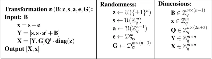
Our randomized transformationϕis shown inFigure 1. The transformation uses, as randomness, both

auniformsecret vectorsand abinarysecret vectorz. Informally, the intuition is that bysimultaneously

multiplying bys(on theleft) and byz(on theright), the same transformation is able to produce (depending on how the inputBwas chosen) either

• a binary LWE distribution with secretz(whenBis uniform), or

• a (transposed4) standard LWE distribution with secret[s,St_]t _{(whenB= (AS+E)}t_).

Intuitively, one may think ofϕ as mappingBto[B,Bz+e]. So, whenBis uniformly random,ϕ outputs the binary LWE distribution by construction. On the other hand, ifB= (AS+E)t =StAt+Et, the transformation outputs[B,Bz+e] =St[At,Atz] + [Et,Etz+e], which looks like a standard (transposed) LWE label matrix. In fact, by the Leftover Hash Lemma, one may argue that[At_,At_{z]is statistically}

close to a uniformly distributed matrix. Unfortunately, the error matrix[Et,Etz+e]does not follow the Gaussian distribution5required by LWE. So, in order to address this and other technical difficulties, the actual transformationϕis a bit more complex. The details of the transformation are somewhat technical,

4_{The LWE distributionsBand ˆBare transposed to allow for the multiplication of the uniform secretson the left.} 5_{In particular, the second part of the error matrixE}t_{z+ewill typically have much larger entries thanEˆ, and also be somehow}

Transformationϕ(B;z,s,a,e,G): Input: B

x=s+e

Y= [s,s·at_+B] X= [Y,G]Qt·diag(z)

Output[X,x]

Randomness: z←U({±1}n₎ s←U(Zmq) a←U(Zn−q 1)

e←Dm

2σ

G←Dm×_σ (n+3)

Dimensions: B∈_Zm×q (n−1) x∈_Zm

q

Q∈_Zn×q (2n+3) Y∈Zm×nq

X∈_Zm×n

q

Figure 1: Transformation proving the pseudorandomness of binary LWE, whereQis the matrix specified inLemma 2.7.

and they are primarily motivated by all the cancellations needed for the proof to work and obtain the proper LWE Gaussian error distribution.

One way to gain additional insight into the construction is to notice that the transformationϕ(B)

always outputs a pair[X,x]such thatXz=s+Gv≈s+e=x. (See proof ofClaim 3.2for details.) So, distribution ˆB=ϕ(B)will also satisfy this property with high probability: there must be a small vector

ˆz∈ {±1}n+1_{such that(A ˆSˆ +Eˆ)}t_{ˆz≈0. This shows that the pseudorandom matrixBˆ = (A ˆSˆ +Eˆ)}t _is

already somehow close to a binary LWE instance because there is a±1 combination of the firstncolumns ofBˆ that is close to the last column. In fact, something very similar can be proved directly, without using

ϕ: matrixAˆt maps a set{0,1}n+1 of size 2n>qk+1to a setZkq+1of sizeqk+1. So, by the pigeon-hole

principle, there exist two binary inputs such thatAˆtˆz0=Aˆtˆz1, or, equivalently, a small vectorˆz=ˆz0−ˆz1

(withkzk_∞=1) such thatBˆzˆ =Eˆt_{ˆz≈0. An informal interpretation of this argument (which, in fact, is}

closely related to the proof that LWE is robust with respect to the secret distribution [11]) is that matrix

ˆ

At hashes the binary secretˆzto an almost uniform (smaller dimensional) secretAˆtˆzwith entries inZq.

But, as before, the problem with this intuitive approach is that the error distributionEˆtˆzis not Gaussian, and it is correlated with the secretˆz.

Our theorem below solves these technical problems using a carefully designed gadget matrix Q

(described inLemma 2.7) which efficiently adjusts the error distribution using some extra randomness

G. Notice how, in the process of transforming LWE into binary LWE, the number of samplesn−1 in the presumed hardLWE(q,k×m,n−1,σ)instance becomes the sizenof the secret in the final binary

LWE instanceLWE±(q,n,m,σˆ). Similarly, the number of columnsm(i. e., the number of parallel LWE instances) in the presumed hardLWE(q,(k+1)×m,n+1,2σ)instance becomes the number of samples in the final binary LWE instance.

Theorem 3.1. Assume the distributionsLWE(q,k×m,n−1,σ)andLWE(q,(k+1)×m,n+1,2σ)are pseudorandom. If q≤2nO(1),σ≥ω(

√

logn), k≥ω(logn), and n≥(k+1)·log₂(q) +ω(logn), then the

distributionLWE±(q,n,m,σˆ)is also pseudorandom forσˆ =2σ

√

n+1.

Proof. We useZas a shorthand for the diagonal matrixdiag(z). We first show that the transformationϕ

maps the uniform distribution to the binary LWE distribution.

Proof. We show that for any fixed values ofa∈_Zn−1

q andz∈ {±1}n, the output of the transformation

[X,x] =ϕ(B)is statistically close to theLWE±distribution with secretz, i. e.,X∈Zm×nq is uniformly

random, and the conditional distribution of the noise vectorˆe=x−Xz(givenXandz) is statistically close toDm_σˆ. All this is over the probability space defined by the random choice ofB,s,e,G. The claim follows by averaging overaandz.

LetQ= [Q_[n],Q]n[]be the matrix defined inLemma 2.7, and recall thatQ[n]∈Zn×nis invertible,

utQ[n] =et1, and the vectorv

t _=ut_Q

]n[∈Zn+3 has norm kvk=2 √

n, kvk_∞≤2. Since s andB are uniformly random, the matrixYis also uniformly distributed, and independent ofeandG. SinceQt_[n]

andZare invertible, the matrix

X= [Y,G][Q[n],Q]n[]tZ=Y(Qt[n]Z) + (GQ

t

]n[Z)

is also uniformly distributed, independently ofG,e. It remains to analyze the conditional distribution of the error vectorˆe=x−Xz. UsingZ·z=uandYQt

[n]u=Ye1=s, we getXz=YQ

t

[n]u+GQ

t

]n[u=s+Gv.

So, the error vector equals ˆe= (s+e)−Xz=e−Gv. Since the entries ofGandeare independent discrete Gaussians of parameterσ and 2σ (respectively), the coordinates ofˆeare independent identically

distributed random variables, each following the distribution D2σ−∑iviDσ. By Lemma 2.5, this

distribution is statistically close toDσˆ for

ˆ

σ=

r

(2σ)2+

_∑

i

(viσ)2=σ

q

4+kvk2_=2σ√_n+1.

Next, consider the output[X,x]whenBfollows distributionB.

Claim 3.3. The distributionϕ(B)is statistically close toBˆ.

Proof. LetB= (AS+E)t forA←U(Zq(n−1)×k),S←U(Zk×mq )andE←D

(n−1)×m

σ . By linearity, we can

writeY= [s,sat+B] =Ys+Yeas the sum of two matrices

Ys= [s,sat+StAt] and Ye= [0,Et].

Similarly, we can also decomposeϕ(B) = [X,x] = [Xs,s] + [Xe,e]as a sum where

Xs=YsQt_[n]Z and Xe= [Ye,G]QtZ= [Et,G]Qt_]1[Z.

Our goal is to show that[Xs,s]t_{=A ˆSˆ and[Xe,e]}t_{=Eˆ forA,ˆ ˆS,Eˆ distributed as in the definition of ˆB.}

We first look at the distribution of the error matrixEˆt = [Xe,e]. The last columne is a discrete Gaussian of parameter 2σby construction. Since[Et,G]has Gaussian distributionDm×σ (2n+2), the rest of

the matrix is distributed according to

Xte←Z t

Q]1[(D

(2n+2)×m

σ )≈Z(D

n×m

2σ ) =D

n×m

2σ ,

for any fixed value ofz, where we have used the propertyQ]1[(D2σn+2)≈D

n

2σ fromLemma 2.7, and the

symmetryZDn_2σ =Dn_2σ. This proves thatEˆ has Gaussian distribution of parameter 2σ, and it depends

We now look at the distribution of[Xs,s] = (A ˆSˆ )t over the random choice ofa,s,z,AandS. The idea is to setˆS= [s,St]t, so that ˆSis distributed uniformly at random overZ(qk+1)×m. But, in order to properly

randomizeAˆ, we define

ˆS=W−1

st S

where W is a uniformly random invertible matrix in Zq(k+1)×(k+1). Since W is invertible, ˆS is still

uniformly distributed, and independent ofW. Next, define

ˆ

A=

I zt

ZQ_[n]HW∈Z

(n+1)×(k+1)

q where H=

1 0t

a A

∈_Zn×q (k+1).

Using the identitieszt_ZQ

[n]=utQ[n] =et1andHW ˆS=H[s,St]t =Yts, we see that our choice ofA,ˆ ˆS

satisfies(A ˆSˆ )t _{= [Xs,s]as desired. All that is left to do is to prove thatAˆ is statistically close to uniform,}

independently of ˆS. We first look atHW. Letwt be the first row ofW. That’s also the first row ofHW. The remaining rows ofHWare [a,A]W. The first rowwt is distributed uniformly at random among all primitive vectors inZkq+1, i. e., all vectors such that gcd(w,q) =1. So, byLemma 2.2, the vectorw

is within negligible statistical distance from the uniform distribution overZkq+1. Finally, since[a,A]is

uniform by construction, andWis invertible, the bottom rows ([a,A]W) ofHWare uniform too, and independent ofw. So,HWis statistically close to uniform overZqn×(k+1). The matrixAˇ = (ZQ[n]HW)t

is also statistically close to uniform (and independent ofz) becauseQ_[n] andZare invertible. Finally,

using the Leftover Hash Lemma (Lemma 2.1) and the assumptionn≥(k+1)log₂(q) +ω(logn), we

see thatAˆt =Aˇ[I,z] = [A,ˇ Azˇ ]is also statistically close to uniform. This concludes the proof that

ϕ(B) = (A ˆSˆ +Eˆ)t whereA,ˆ ˆSandEˆ follow the LWE distribution as in the definition of ˆB.

We are now ready to prove the theorem. It follows from pseudorandomness of theLWE(q,k×m,n− 1,σ)that the distributionBis computationally indistinguishable from the uniform distributionUover

Zm×q (n−1). Sinceϕis efficiently computable, the distributionsϕ(B)andϕ(U)are also computationally

indistinguishable. ByClaim 3.2, ϕ(U) is statistically close to LWE±(q,n×1,m,σˆ). Similarly, by

Claim 3.3,ϕ(B)is statistically close to ˆB. So,LWE±(q,n×1,m,σˆ)is computationally indistinguishable

from ˆB. Finally, from the pseudorandomness of LWE(q,(k+1)×m,n+1,2σ), we know that the

distribution ˆBis computationally indistinguishable from the uniform distribution overZm×q (n+1). It follows

by transitivity that the binary LWE distributionLWE±(q,n,m,σˆ)is computationally indistinguishable from the uniform distribution overZm×q (n+1), i. e.,LWE±(q,n,m,σˆ)is pseudorandom.

The statement in the above theorem can be simplified usingLemma 2.9to rephrase it in terms of the basic LWE problem, and by noticing thatLWE(q,k,n,σ)does not get any easier whenkandσgrow, or

whenngets smaller.

Corollary 3.4. Assume the distributionLWE(q,k,n+1,σ)is pseudorandom for some q≤2nO(1),σ ≥ ω(

√

logn), k≥ω(logn), and(n+1)≥(k+1)·(log₂(q) +1). Then the distributionLWE±(q,n,nO(1),σˆ)

is also pseudorandom forσˆ =2σ

√

Proof. Notice that, under the assumptions in the corollary statement,

n≥(k+1)log₂q+k≥(k+1)log₂q+ω(logn)

as required byTheorem 3.1. In order to invoke the theorem, we also need to verify the pseudorandomness conditions. AssumeLWE(q,k,n+1,σ)is pseudorandom. Dropping the last two rows from the samples

[A,b]←LWE(q,k,n+1,σ)shows thatLWE(q,k,n−1,σ)is also pseudorandom. The samples[A,b]

can also be mapped toLWE(q,k+1,n+1,2σ)by performing the following two operations:

• Add an extra Gaussian error terme←Dn_√+1

3σ tob. ByLemma 2.5, this has the effect of increasing

the error rate to√σ2+3σ2=2σ.

• Append an extra columnatoAand add a random multiplea·stob. This has the effect of extending the secret with an extra coordinates.

Since this transformation also preserves the uniform distribution, it provides a reduction from

LWE(q,k,n+1,σ) to LWE(q,k+1,n+1,2σ),

and proves thatLWE(q,k+1,n+1,2σ)is pseudorandom. Finally, byLemma 2.9,

LWE(q,k×m,n−1,σ) and LWE(q,(k+1)×m,n+1,2σ)

are also pseudorandom, as required byTheorem 3.1.

Notice howCorollary 3.4establishes the pseudorandomness ofLWE±for any polynomial number of samplesm=nO(1), using, as an assumption, only the pseudorandomness ofLWEfor a fixed number (n+1≈klogq) of samples. (This property is also implicit in [6].) We remark that we phrasedTheorem 3.1

andCorollary 3.4asymptotically (in terms of polynomial-time distinguishers achieving at most negligible advantageε=n−ω(1)) only for simplicity. All statements and proofs are easily adapted to other settings,

e. g., to prove hardness of binary LWE against adversaries running in subexponential time.

4

Conclusion

We presented a simple proof that the LWE problem with binary secret of sizen=O(klog₂q)is as hard as LWE with uniformly random secret inZkq. More specifically, if LWE with secrets inZkqandn≈klogq

samples is pseudorandom, then LWE with secrets in{0,1}n _or{±1}n _{(and an arbitrary polynomial}

number of samplesnO(1)) is also pseudorandom. As already observed in [6], the growth in the dimension of the secret is seemingly optimal, because it approximately preserves the bit-size of the secret, and the cost of a brute force attack. Starting from LWE with a fixed number of samplesm≈klogq=O(klogk)

can be given starting from LWE with an even smaller number of samples, e. g.,m=O(k)linear in the secret dimension.

An important open problem is whether similar results can be proved for the structured variants of LWE based on algebraic lattices [15,14]. The use of structured lattices is of primary importance to make lattice cryptography efficient in practice, and the use of LWE with binary secrets plays an important role in some applications, like Fully Homomorphic Encryption schemes [9,8], to control the noise growth when computing on encrypted data. We remark that the use of binary secrets and errors does not seem to pose any difficulty in the setting of one-way hash functions based on structured lattices [15]. However, for LWE [21,14], it is unclear how to adapt the proof in this paper to the algebraic lattice setting. We hope our simple proof for unstructured lattices will bring more attention to this problem, and serve as a possible starting point to establish similar results for ring LWE.

Acknowledgments. The author thanks the anonymous Theory of Computing referees and editor Oded

Regev for useful comments on earlier drafts of this paper.

References

[1] MARTINR. ALBRECHT: On dual lattice attacks against small-secret LWE and parameter choices in HElib and SEAL. InProc. 36th Ann. Internat. Conf. on the Theory and Applications of Cryp-tographic Techniques (EUROCRYPT’17), pp. 103–129. Springer, 2017. [ doi:10.1007/978-3-319-56614-6_4] 3

[2] MARTINR. ALBRECHT, CARLOSCID, JEAN-CHARLESFAUGÈRE, ROBERTFITZPATRICK,AND

LUDOVIC PERRET: Algebraic algorithms for LWE problems. ACM Comm. Computer Algebra, 49(2):62, 2015. [doi:10.1145/2815111.2815158] 3

[3] BENNYAPPLEBAUM, DAVIDCASH, CHRISPEIKERT,ANDAMIT SAHAI: Fast cryptographic primitives and circular-secure encryption based on hard learning problems. InProc. 29th Ann. Internat. Crypto. Conf. (CRYPTO’09), pp. 595–618. Springer, 2009. [ doi:10.1007/978-3-642-03356-8_35] 2

[4] SANJEEVARORA ANDRONGGE: New algorithms for learning in presence of errors. InProc. 38th Internat. Colloq. on Automata, Languages and Programming (ICALP’11), pp. 403–415. Springer, 2011. [doi:10.1007/978-3-642-22006-7_34] 3

[5] SHIBAI ANDSTEVEND. GALBRAITH: Lattice decoding attacks on binary LWE. InProc. 19th Australasian Conf. on Information Security and Privacy (ACISP’14), pp. 322–337. Springer, 2014. [doi:10.1007/978-3-319-08344-5_21] 3

[6] ZVIKA BRAKERSKI, ADELINE LANGLOIS, CHRIS PEIKERT, ODED REGEV, AND DAMIEN

[7] JOHANNES A. BUCHMANN, FLORIANGÖPFERT, RACHELPLAYER,ANDTHOMASWUNDERER: On the hardness of LWE with binary error: Revisiting the hybrid lattice-reduction and meet-in-the-middle attack. InProc. 8th Internat. Conf. on Progress in Cryptology (AFRICACRYPT’16), pp. 24–43. Springer, 2016. [doi:10.1007/978-3-319-31517-1_2] 3

[8] ILARIACHILLOTTI, NICOLASGAMA, MARIYAGEORGIEVA,ANDMALIKAIZABACHÈNE: Faster fully homomorphic encryption: Bootstrapping in less than 0.1 seconds. InProc. 22nd Internat. Conf. on the Theory and Application of Cryptology and Information Security (ASIACRYPT’16), pp. 3–33. Springer, 2016. [doi:10.1007/978-3-662-53887-6_1] 2,15

[9] LÉODUCAS ANDDANIELE MICCIANCIO: FHEW: Bootstrapping homomorphic encryption in less than a second. InProc. 34th Ann. Internat. Conf. on the Theory and Applications of Cryptographic Techniques (EUROCRYPT’15), pp. 617–640. Springer, 2015. [doi:10.1007/978-3-662-46800-5_24]

2,15

[10] CRAIGGENTRY, CHRIS PEIKERT,ANDVINODVAIKUNTANATHAN: Trapdoors for hard lattices and new cryptographic constructions. In Proc. 40th STOC, pp. 197–206. ACM Press, 2008. [doi:10.1145/1374376.1374407] 5

[11] SHAFIGOLDWASSER, YAELTAUMANKALAI, CHRISPEIKERT,ANDVINODVAIKUNTANATHAN: Robustness of the learning with errors assumption. InProc. 1st Conf. on Innovations in Theoret. Computer Science (ITCS’10), pp. 230–240. Tsinghua University Press, 2010. 2,3,11

[12] JOHANHÅSTAD, RUSSELLIMPAGLIAZZO, LEONIDA. LEVIN,ANDMICHAELLUBY: A pseu-dorandom generator from any one-way function. SIAM J. Comput., 28(4):1364–1396, 1999. [doi:10.1137/S0097539793244708] 4

[13] PAUL KIRCHNER ANDPIERRE-ALAIN FOUQUE: An improved BKW algorithm for LWE with applications to cryptography and lattices. InProc. 35th Ann. Internat. Crypto. Conf. (CRYPTO’15), pp. 43–62. Springer, 2015. [doi:10.1007/978-3-662-47989-6_3,arXiv:1506.02717] 3

[14] VADIM LYUBASHEVSKY, CHRISPEIKERT,ANDODED REGEV: On ideal lattices and learning with errors over rings. J. ACM, 60(6):43:1–43:35, 2013. Preliminary version inEUROCRYPT’10. [doi:10.1145/2535925] 15

[15] DANIELE MICCIANCIO: Generalized compact knapsacks, cyclic lattices, and efficient one-way functions. Comput. Complexity, 16(4):365–411, 2007. Preliminary version in FOCS’02. [doi:10.1007/s00037-007-0234-9] 15

[16] DANIELEMICCIANCIO ANDPETROSMOL: Pseudorandom knapsacks and the sample complexity of LWE search-to-decision reductions. InProc. 31st Ann. Internat. Crypto. Conf. (CRYPTO’11), pp. 465–484. Springer, 2011. [doi:10.1007/978-3-642-22792-9_26] 8

[18] DANIELE MICCIANCIO AND ODED REGEV: Worst-case to average-case reductions based on Gaussian measures. SIAM J. Comput., 37(1):267–302, 2007. Preliminary version inFOCS’04. [doi:10.1137/S0097539705447360] 5

[19] CHRISPEIKERT: Public-key cryptosystems from the worst-case shortest vector problem: extended

abstract. InProc. 41st STOC, pp. 333–342. ACM Press, 2009. [doi:10.1145/1536414.1536461] 8

[20] CHRISPEIKERT, ODEDREGEV,ANDNOAHSTEPHENS-DAVIDOWITZ: Pseudorandomness of ring-LWE for any ring and modulus. In Proc. 49th STOC, pp. 461–473. ACM Press, 2017. [doi:10.1145/3055399.3055489] 8

[21] ODEDREGEV: On lattices, learning with errors, random linear codes, and cryptography.J. ACM, 56(6):34:1–34:40, 2009. Preliminary version inSTOC’05. [doi:10.1145/1568318.1568324] 1,8,15

[22] ODED REGEV: The learning with errors problem (invited survey). In Proc. 25th Conf. on Computational Complexity (CCC’10), pp. 191–204. IEEE Comp. Soc. Press, 2010. [doi:10.1109/CCC.2010.26] 1

AUTHOR

Daniele Micciancio Professor

University of California at San Diego (UCSD) La Jolla, CA, USA

daniele cs ucsd edu

http://cseweb.ucsd.edu/~daniele/

ABOUT THE AUTHOR