Copyright © The Author(s). All Rights Reserved. Published by American Research Institute for Policy Development DOI: 10.15640/ijhs.v7n3a3 URL: https://doi.org/10.15640/ijhs.v7n3a3
Random Power Function of Bent-cable Growth Models for Longitudinal Data: Application
to AIDS Studies
Getachew A. Dagne
1Abstract
This paper presents a power function within a bent-cable model for identifying a transition period for the development of drug resistance to antiretroviral treatment (ART) in HIV/AIDS studies or other related fields. Such a transition period usually occurs between incoming and outgoing phases of trajectories of longitudinal data. The transition curve is modeled using a power function with unknown width, and we assess this clinically important feature of the longitudinal HIV/AIDS data using the bent-cable framework with random subject-specific parameters, including parameters of the transition curve. We develop a fully Bayesian approach for fitting a power function of bent-cable Tobit model to left-censored data and illustrate the proposed methods on real data from an AIDS clinical study.
Keywords: Bayesian inference; change-points; longitudinal study; mixed-effects models; skew distribution 1. Introduction
Very often longitudinal studies produce outcome variables whose trajectories may exhibit several phasic changes over time. Characterizing and identifying those phases of trajectories is important in clinical practice. For example, in longitudinal clinical studies of the efficacy of antiretroviral (ARV) drugs, typical trajectories of viral load (number of HIV RNA copies in plasma) of patients, after receiving ARV, initially start declining (phase 1) then followed by a gradual transition period (phase 2), and finally a third phase of upward (rebound), predicting progression to AIDS (Paterson et al., 2000; Dagne, 2018). These different phases may occur because of a biological process of developing resistance to ARV drugs and non-adherence over time (Paterson et al., 2000). To describe the phasic patterns, one can use a bent-cable model (Chiua et al., 2006). The transition phase in the regular bent-cable model is modeled using a quadratic function which may be too restrictive for adequately describe it. In this paper, we develop a bent-cable model by jointly (i) relaxing the assumption of the quadratic function for the transition period, (ii) allowing subject-to-subject variability in the parameters of the proposed model, (iii) incorporating skewness and detection limits in a distribution of viral loads(Wu and Zhang, 2002), and (iv) adjusting for measurement errors in covariates.
In assessing subject-specific growth curves (trajectories) of a longitudinal response, the features of the data determine the types of models to be adopted. In cases where there are abrupt changes in trajectories, piecewise or ``broken-stick'' models are usually effective (Kiuchi et al., 2001; Slate et al., 2001; Hall et al., 2003; Zhao et al., 2015). In other cases where there are smooth and gradual transitions between incoming and outgoing phases, a power function of bent-cable model is preferred (Khan and Kar, 2018) instead of a piecewise model. For instance, in the case of HIV/AIDS studies, growth curves of longitudinal data may show gradual transition periods between an initial decline in viral load after treatment and rebound at later time in the study. These growth curves also exhibit subject-to-subject variability, and assuming fixed parameters instead of random may not reflect the biological reality. To properly analyze such data, we use a random power function of bent-cable model (see Section 2 for details) which also incorporates statistical adjustments for measurement error in covariates and left-censoring due to lower detection limit (LOD).
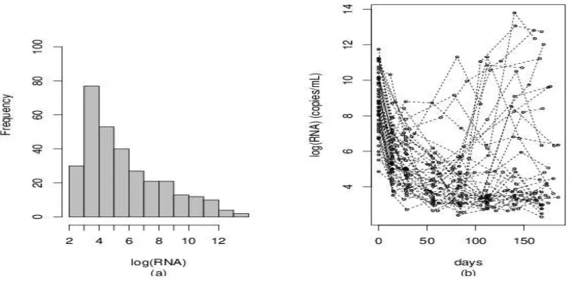
Fig. 1: (a) Histogram of log viral load; (b) spaghetti plot of log viral load
Often viral load data suffer from left-censoring and skewness. To account for left-censoring within the power function of bent-cable model, we jointly use the Tobit model (Tobin, 1958) which provides consistent estimates of parameters. The commonly used Tobit model assumes normality which may not be suitable for a highly skewed distribution of viral load measurements (Dagne, 2018). For example, Figure 1(a) shows the histogram of viral loads for patients enrolled in the AIDS clinical trial study--A5055 (Acosta et al., 2004). From the histogram one can observe that the distribution of log-transformed viral load data exhibit right skewness. In this paper, we use skew-elliptical distributions (Sahu et al., 2003; Genton, 2004), where multivariate skew-normal (SN) and multivariate skew-t (ST) distributions are special cases, for modeling left-censored HIV-RNA data with phasic patterns. In Section 2, we develop a power function of bent-cable Tobit models with multivariate ST distributions in full generality. In Section 3, we present the Bayesian inferential procedure. The proposed methodologies are illustrated using the AIDS data set in Section 4. Finally, the paper concludes with discussions in Section 5.
2. Power Function of Bent-cable Growth Models 2.1. Motivating data
The motivating data for our paper were obtained from an AIDS clinical trial study (A5055) (Acosta et al., 2004). Forty four HIV-1 infected patients were treated with a potent ARV regimen with a combined use of a protease inhibitor, nelfinavir (2,250 mg/d), and transcriptase inhibitors, zidovudine (600 mg/d) and lamivudine (300 mg/d). The outcome variable was RNA viral load (copies/mL), recorded at 0, 7, 14, 28, 56, 84, 112, 140 and 168 days of follow-up. CD4 cell counts were also measured. The number of observations varies from patient to patient with a median of 8 measurements and a standard deviation of 1.49. Figure 1(b) depicts the trajectories of log viral load over time, showing some phasic patterns. These patterns comprise an initial decreasing trend, a gradual transition part and an increasing upward trend for a typical patient. Modeling these patterns has clinical importance for assessing the effectiveness of ARV drugs and AIDS progression. In the modeling process, we also take into account left-censoring of viral load (detectable lower limit is 50 copies/mL) by using a Tobit model which is discussed in the next section. 2.2.Model specification
We now develop a power function of bent-cable Tobit model (PBTM) which simultaneously incorporates left-censoring, skewness and measurement errors in covariates. The outcome variable for our study is denoted by𝑦𝑖𝑗∗,
and 𝑧𝑖𝑗∗ be a true covariate for the individual i at time 𝑡
𝑖𝑗 (i=1,2,…,n; j=1,2,…,𝑛𝑖). Let 𝑐𝑖𝑗 = 0 if 𝑦𝑖𝑗∗is observed (above
the lower detection limit (LOD)) and 𝑐𝑖𝑗 = 1 if 𝑦𝑖𝑗∗is left-censored (below LOD). Some of the observed values of the
outcome variable may be recorded as being equal to or below LOD due to left-censoring, making them unreliable. To distinguish these measurements, we define an indicator 𝑐𝑖𝑗 = 0 if 𝑦𝑖𝑗∗is observed and 𝑐𝑖𝑗 = 1 if 𝑦𝑖𝑗∗ is left-censored. A
Tobit model (Tobin, 1958) is adopted for modeling such left-censored longitudinal data as follows.𝑦𝑖𝑗 = 𝑦𝑖𝑗∗𝑖𝑓𝑦𝑖𝑗∗ >
The main focus of PBTM is on modeling longitudinal data with multiple phasic patterns based on an ST distribution for 𝑦𝑖𝑗 as follows
𝑦𝑖𝑗 = 𝑔 𝑡𝑖𝑗, 𝜇𝑖𝑗, 𝑧𝑖𝑗∗ + 𝑒𝑖𝑗𝑒𝑖 ∼ 𝑆𝑇𝑛𝑖, 𝜈𝑒(0, 𝜎𝑒2𝐼𝑛𝑖,Δ(𝛿𝑒𝑖)) (2)
Where𝜇𝑖𝑗 is the mean structure, and the error𝑒𝑖 = (𝑒𝑖1, … , 𝑒𝑖𝑛𝑖)′follows a multivariate ST distribution with degrees of freedom 𝜈𝑒, variance 𝜎𝑒2 and 𝑛
𝑖× 𝑛𝑖skewness diagonal matrix Δ(𝛿𝑒𝑖)= 𝛿𝑒𝐼𝑛𝑖.
The mean structure 𝜇𝑖𝑗 in (2) is a power function of bent-cable model to assess multiple phases of trajectories
such as: (i) incoming trend, (ii) outgoing trend, and (iii) transition power function that connects the incoming and outgoing trends. The power function, where a quadratic function is a special case (Chiua et al., 2006; Khan et al, 2009), represents the gradual transition period between two unknown time points 𝑇1𝑖 and 𝑇2𝑖. Following Khan and Kar (2018), suppose 𝑇1𝑖= 𝜙1𝑖− 𝜙2𝑖(𝜙3𝑖− 1) and 𝑇2𝑖= 𝜙1𝑖+ 𝜙2𝑖, such that 𝑇1𝑖<𝜙1𝑖<𝑇2𝑖 and 𝜙1𝑖, 𝜙2𝑖> 0, and 𝜙3𝑖> 1.These parameters can also be considered as random coefficients in the mean structure of PBTM (Tishler et al., 1981; Chiua et al., 2006) as follows.
The mean 𝜇𝑖𝑗 is modeled as 𝜇𝑖𝑗 = 𝜂𝑧𝑖𝑗∗ + 𝛽
1𝑖+ 𝛽2𝑖𝑡𝑖𝑗 + 𝛽3𝑖𝑞(𝑡𝑖𝑗, 𝜅𝑖) (3)
where 𝜂 measures the effect of time-varying covariate;
𝑞 (𝑡𝑖𝑗, 𝜅𝑖 = 𝜙2𝑖(𝑡𝑖𝑗 − 𝜙1𝑖 𝜙3𝑖− 1 )/(𝜙2𝑖𝜙3𝑖))^𝜙3𝑖𝐼 (𝜙1𝑖− 𝜙2𝑖 𝜙3𝑖− 1 < 𝑡𝑖𝑗 ≤ 𝜙1𝑖+ 𝜙2𝑖) + (𝑡𝑖𝑗 −
𝜙1𝑖)𝐼(𝑡𝑖𝑗 > 𝜙1𝑖+ 𝜙2𝑖) I(.) is an indictor function;𝛽1𝑖 and 𝛽2𝑖are the incoming random intercept and slope, respectively; 𝛽3𝑖is the change in slope between the incoming and outgoing linear phases; 𝜅𝑖=(𝜙1𝑖𝜙2𝑖, 𝜙3𝑖}) are the parameters of the power function, 𝑞(𝑡𝑖𝑗, 𝜅𝑖), which presents the transition phase. Note that the power function of
the bent-cable model becomes an ordinary bent-cable when 𝜙3𝑖=2 and a broken-stick model when 𝜙2𝑖= 0, 𝜙3𝑖> 1 or 𝜙2𝑖> 0, 𝜙3𝑖= 1.
The random parameters in (3) are modeled as
𝛽1𝑖= 𝛽1+ 𝑏1𝑖 , 𝛽2𝑖 = 𝛽2+ 𝑏2𝑖 , 𝛽3𝑖 = 𝛽3+ 𝑏3𝑖 (4) 𝜙1𝑖 = 𝜙1+ 𝑏4𝑖, 𝜙2𝑖 = 𝜙2+ 𝑏5𝑖, 𝜙3𝑖 = 𝜙3+ 𝑏6𝑖 Where𝛽 = (𝛽1, 𝛽2, 𝛽3, 𝜙1, 𝜙2, 𝜙3)′ are population-based parameters. The random effects
(𝑏1𝑖, … , 𝑏6𝑖)′have a multivariate normal distribution 𝑁(0,Σ𝑏) where Σ𝑏 is a variance-covariance matrix with
dimension of 6. The critical time point, where the mean trajectory shifts from a decreasing trend to an upward trend, is located at 𝜒 = 𝜙1 𝜙3− 1 𝜙2+ 𝛽2
𝛽3 𝜙2𝜙3
𝜙2−1 − 𝜙3−1 (Khan and Kar, 2018). In the estimation process
of these parameters of the power function of bent-cable Tobit model in (3), measurement errors in covariates (e.g., CD4) (Raboud et al., 1996) are also addressed. Next, we present a covariate measurement error model.
2.3. Covariate measurement error models
For explaining some of the variations of the outcome variable of PBTM, time-varying covariates such as CD4 cell counts are used. It is often the case that CD4 cell counts are measured with errors (Higgins et al., 1997; Wu, 2002; Carroll et al., 2006). To incorporate measurement errors, we adopt a polynomial mixed-effects model as follows.
𝑧𝑖𝑗 = 𝑢𝑖𝑗𝛼 + 𝑣𝑖𝑗𝑎𝑖+ 𝜖𝑖𝑗, 𝜖𝑖∼ 𝑆𝑇_𝑛𝑖𝜈𝑧(0, 𝜎𝑧2𝐼
𝑛𝑖,Δ(𝛿𝜖𝑖)) (5)
Where𝑧𝑖𝑗is the observed CD4 cell count with measurement errors for individual i
at time 𝑡𝑖𝑗 and let 𝑧𝑖𝑗∗ = 𝑢
𝑖𝑗𝛼 + 𝑣𝑖𝑗𝑎𝑖 be the trueCD4 cell count at time 𝑡𝑖𝑗,
𝑢𝑖𝑗and𝑣𝑖𝑗 are 1 × 𝑙design vectors, 𝛼 = (𝛼1, … , 𝛼𝑙)′ and 𝑎𝑖 = (𝑎𝑖1, … , 𝑎𝑖𝑙)′ are fixed-effects and random-effects parameter vectors, respectively. We assume that𝑎𝑖 ∼ 𝑁𝑙(0,Σ𝑎), where
Σ𝑎is a covariance matrix. Here, we consider the model in (5) with𝑢𝑖𝑗 = 𝑣𝑖𝑗 = 1, 𝑡𝑖𝑗, … , 𝑡𝑙−1𝑖𝑗 , and AIC and BIC
3. Bayesian estimation
The model parameters of models in (2) and (5) are estimated using a Bayesian approach. To facilitate the estimation, we use the stochastic representation for the ST distribution by introducing an𝑛𝑖× 1 random variable vector 𝑤𝑖= (𝑤𝑖1, … , 𝑤𝑖𝑛𝑖)′ and 𝜉𝑒𝑖as a scaling weight (Sahu et al., 2003; Dagne, 2017). Such a representation makes the use of Bayesian algorithms simpler as given below.
𝑦𝑖𝑗 ∼ 𝑁 𝑔 𝑡𝑖𝑗, 𝜇𝑖𝑗, 𝑧𝑖𝑗∗ + 𝛿𝑒𝑖𝑗𝑤𝑒𝑖𝑗, 𝜉𝑒−1𝑖 𝜎𝑒2 , 𝑤𝑒𝑖𝑗 ∼ 𝑁 0,1 𝐼 𝑤𝑒𝑖𝑗 > 0 , 𝜉𝑒𝑖𝑗 ∼ 𝐺
𝜈𝑒 2 ,
𝜈𝑒 2 𝑧𝑖𝑗 ∼ 𝑁 𝑧𝑖𝑗∗ + 𝛿
𝜖𝑖𝑗𝑤𝜖𝑖𝑗, 𝜎𝑧2 , 𝑎𝑖 ∼ 𝑁𝑙 0,Σ𝑎 , 𝑏𝑖∼ 𝑁6 0,Σ𝑏 (6)
where G(.) is a gamma distribution, 𝐼(𝑤𝑒𝑖𝑗 > 0) is an indicator with𝑤𝑒𝑖𝑗 ∼ 𝑁(0,1) and 𝑤𝑒𝑖𝑗 > 0.𝑧𝑖𝑗∗isthe
true but unobservable covariate value at time 𝑡𝑖𝑗. The ST distribution (6) can be reduced to the following three special
cases: (i) a skew-normal (SN) distribution as 𝜈𝑒 →∞ and 𝜉𝑒𝑖 → 1 with probability 1, (ii) a standard t-distribution as 𝛿𝑒𝑖𝑗 = 0, or (iii) a standard normal distribution as𝜈𝑒 →∞ $\ and 𝛿𝑒𝑖𝑗 = 0 .
Let 𝜃 = (𝛼, 𝛽, 𝜂, 𝜎𝑧2, 𝜎
𝑒2,Σ𝑎,Σ𝑏, 𝜈𝑒,Δ𝑒𝑖, 𝑖 = 1, … , 𝑛) be the unknown parameters in models (2, 5) with the joint prior
distribution𝑔 𝜃 where assessments of specific prior distributions are given in Section 4.
Statistical inference for the parameters of the proposed models is carried out using their posterior distributions, which are obtained by combining the likelihood of the observeddata and the prior distributions via the Bayes' theorem. Let f(.|.) and F(.|.) denote a probability distribution and cumulative distribution, respectively. For a left-censored response, a detectable observed value 𝑦𝑖𝑗contributes 𝑓(𝑦𝑖𝑗), while a non-detectable value
contributes𝐹(𝜌) inthe likelihood. Based on this formulation of the likelihood, the jointposterior density of 𝜃based on the observeddata 𝐷 = (𝑦𝑖, 𝑧𝑖, 𝑖 = 1, … , 𝑛) can be given by
𝑓 𝜃 𝐷 ∝
𝑔 𝜃 ∫ ∫ [1 −𝑛𝑖
𝑗 𝑛 𝑖
Pr𝑆𝑖𝑗=1)𝑓𝑦𝑖𝑗1−𝑐𝑖𝑗1−Pr𝑆𝑖𝑗=1+Pr𝑆𝑖𝑗=1𝐹𝜌𝑐𝑖𝑗𝑓𝑧𝑖𝑗𝑓𝑤𝑒𝑖𝑗𝑤𝑒𝑖𝑗>0𝑓𝑤𝜖𝑖𝑗𝑤𝜖𝑖𝑗>0𝑓𝑎𝑖𝑓𝑏𝑖𝑑𝑎𝑖𝑑𝑏𝑖 (7)
wherePr(𝑆𝑖𝑗 = 1) is the probability that a patient's outcome is left-censored. The posterior function in (7) involves integrals of high dimensions and getting closed form solutions is thus difficult. Alternatively, we can use the Monte Carlo Markov chain (MCMC) algorithm to estimate the parameters in (7).
4. Application to HIV/AIDS data 4.1. Specification of models
We now demonstrate the proposed models by fitting them to a real data set from an AIDS clinical study (Acosta et al., 2004). We fit PBTM given in (2-4) to the the natural logarithm of HIV viral load for the ith subject at time 𝑡𝑖𝑗 (i=1, …, n=44, j=1, …, ni), and here 𝑧𝑖𝑗∗ represents the true value of CD4. To estimate the true values of CD4 cell count, a linear mixed-effects model is adopted as given in (5). In particular, we set𝑢𝑖𝑗 = 𝑣𝑖𝑗 = (1, 𝑡𝑖𝑗, … , 𝑡𝑖𝑗𝑙−1)′, taking linear (l=2), quadratic (l=3) and cubic (l=4) polynomials with corresponding AIC (BIC) values of 799.03 (821.74), 703.56 (744.42) and 766.18 (782.08), respectively. Based on these model criteria values, the best model is a quadratic mixed-effects model for the CD4 process (Dagne, 2019).
𝑧𝑖𝑗 = 𝛼1+ 𝑎𝑖1 + 𝛼2+ 𝑎𝑖2 𝑡𝑖𝑗 + 𝛼3+ 𝑎𝑖3 𝑡𝑖𝑗2 + 𝜖𝑖𝑗, (8)
Where𝑧𝑖𝑗∗ = 𝛼1+ 𝑎𝑖1 + 𝛼2+ 𝑎𝑖2 𝑡𝑖𝑗 + 𝛼3+ 𝑎𝑖3 𝑡𝑖𝑗2, 𝛼 = (𝛼1, … , 𝛼3)′ is a vector of population
(fixed-effects) parameters,𝜖𝑖 = 𝜖𝑖1, … , 𝜖𝑖𝑛𝑖
′∼ 𝑆𝑇
𝑛𝑖,𝜈𝑧(0, 𝜎𝑧2𝐼𝑛𝑖, 𝛿𝜖𝐼𝑛𝑖) and individual-specific random-effects 𝑎𝑖 =
𝑎𝑖1, … , 𝑎𝑖3 ′∼ 𝑁3(0,Σ𝑎). For numerical stability, we standardized the time-varying covariate CD4 cell counts.
(iii) a power function of bent-cable Tobit model with skew-t distributions of random errors (Model III). In all these models, we assess how thetrue time-varying covariates, CD4 cell count, would affect the multiple phases of trajectories.
For fitting these models using a Bayesian approach, the hyperparameters of the prior distributions are assessed as follows. (i) Parameters for fixed-effects are assumed to have a normal distribution N(0, 100) for each element of 𝛼, 𝛽, and 𝜂. (ii) For𝜎𝑒2 and𝜎
𝑧2 we assume inverse gamma prior distributions IG(0.01, 0.01). (iii) For the
variance matrices of the random-effects Σ𝑎andΣ𝑏, we assume inverse Wishart distributions IW(Ω1, 𝜌1) and
IW(Ω2, 𝜌2) with covariance matrices Ω1=diag(.01), Ω2= diag(.01) and 𝜌1=3 and 𝜌2=6, respectively. (iv) The
parameter for the degrees of freedom 𝜈𝑒, it follows a gamma distribution G(1.0,.01). (v) For the skewness parameter 𝛿𝑒, a normal distribution N(0,100) is considered.
After applying the Bayes' theorem to the likelihood function and the prior distributions specified above, Bayesian estimation of parameters using the MCMC algorithm is straightforward. Checking the convergence of the MCMC algorithm was carried out using the tools within the WinBUGS software (Lunn et al., 2000). First, to see how well the MCMC generated chains were mixing (showing convergence), we inspected trace plots of the iteration number against the values of the draw of parameters at each iteration. Upon inspection and taking in consideration of the complexity of the power function of bent-cable models, some generated values for some parameters took longer iterations to converge. Convergence was getting better after 100,000 iterations, and thus the first 100,000 iterations were ignored as burn-in. Second, the computed autocorrelations were small after using a thinning of 50, suggesting a good mixing. Third, the Markov chain (MC) errors were less than 5\% of posterior standard deviation values for the parameters, showing good precision and convergence of MCMC (Ntzoufras, 2009). Fourth, the Gelman-Rubin potential scale reduction factors were close to 1 with a range of 1-1.2, confirming convergence. Finally, we retained 10,000 MCMC samples for the purpose of making posterior inference of the unknown parameters of interest. The computational burden to run MCMC for Model II was close to 6 hours on Latitude E5540, Intel(R) Core(TM)i7-4600U @2.10GHz.
4.2. Results of model fit 4.2.1. Model comparison
For choosing the best model out of the three models mentioned above, the values of the Bayesian model selection criteria are presented in Table 1. Accordingly,Model I has the biggest values of deviance (1254.0), RSS (230.649), EPD (2.577), and DIC (1110.820) the second largest values of deviance (988.8), RSS (4.308), EPD (.327), and DIC (822.071) belong to Model III. Model II has the least values of deviance (919.5), RSS (2.108), EPD (.326) and of DIC (631.709), indicating that the skew-normal gives the best fit.
Table 1. Model comparison using Bayesian model selection criteria(RSS=residual sum of squares, EPD= expected predictive deviance, DIC= deviance information criterion)
Criterion ModelI ModelII ModelIII Deviance 1254.0 919.5 988.8 RSS 230.649 2.108 4.308 EPD 2.647 0.326 0.327 DIC 1110.820 631.709 822.071
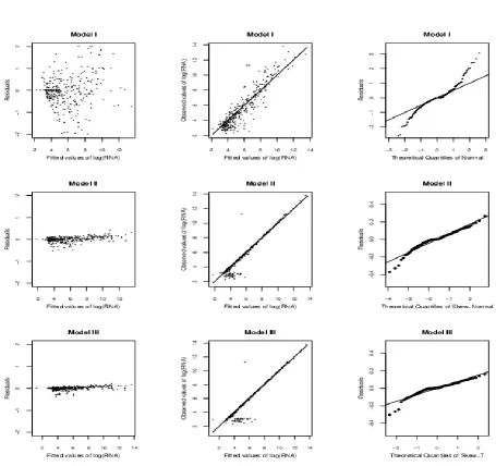
Fig. 2. Plots of goodness-of-fit statistics for three Models: (i) The first column has the residual plots against the fitted values, (ii) the second has plots of the fitted against observed log(RNA) values, and (iii) the last column has the Q-Q plots of residuals.
4.2.2. Bayesian inference under Model II
The best model, Model II, describes well the phasic patterns of viral trajectories by using a power function of the bent-cable with a skew-normal distribution for the error terms. The posterior values of the parameters of Model II are reported in Table 2, specifically in the middle row. The posterior means for the intercept and slope parameters of the incoming trend are𝛽1 = 4.102 and 𝛽2 = -1.27, respectively; for𝛽3, which represents the change in slope between the incoming trend and outgoing trend, the posterior mean is 𝛽3= 1.621$. For the parameters of the power function which represents the transition phase, the posterior means are𝜙1 = 6.886, 𝜙2 = 8.958, 𝜙3= 2.207. The fitted power function of the bent-cable curve is displayed in Figure 3.
From the graph we observe that patients, after receiving the ARV treatment, encounter a decrease in viral load followed by a gradual transition period up until 𝜙1+ 𝜙2= 15.84 weeks. This means that after receiving a
Right after approximately 16 weeks inthe study (the rightdotted line in Figure 3, patients encountered a linear increase at the rate of 1.621 per week. Also, the time point at which the mean trajectory of viral load turns to an upward direction from a decreasing trend is estimated to be 12.225 weeks after the initiation of treatment. In summary, after receiving a treatment, the estimated mean growth trajectory of viral load suggests that the effect of the ARV treatment declines over time by not providing protection against the production of HIV virus. This explains why we see the upward trend towards the end of the study. For Model II, the posterior mean of the variance parameter 𝜎𝑒2, .164, is relatively small implying that taking into account skewness is beneficial. The posterior mean of the
skewness parameter (𝛿𝑒) is 1.81 with a 95% credible interval of (1.257, 2.508), confirming that the use of skewed distributions is very useful. The effect of CD4 on viral load is negative and strong ( 𝜂 = -.893, 95% CI: (-1.337,-.485)), suggesting that as CD4 cell count gets lower, viral load rebounds.
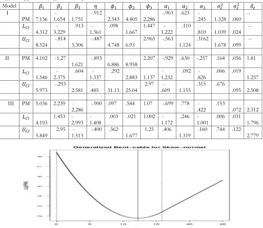
Table 2. A summary of the posterior means (PM) of population parameters along with the corresponding lower limit ( 𝐿𝐶𝐼) and upper limit (𝑈𝐶𝐼) of 95% equal-tail credible interval.
Model 𝛽1 𝛽2 𝛽3 𝜂 𝜙1 𝜙2 𝜙3 𝛼1 𝛼2 𝛼3 𝜎𝑒2 𝜎
𝑧2 𝛿𝑒
I
PM 7.136 -1.654 1.751 -.912 2.343 4.405 2.286 -.903 .623 -.245 1.328 .060 -- 𝐿𝐶𝐼
4.312 -3.229 .913 -1.361 .098 1.667 1.447 -1.222 .110 -.810 1.039 .024 -- 𝑈𝐶𝐼
8.524 -.814 3.306 -.487 4.748 6.93 2.965 -.563 1.124 .3162 1.678 .099 --
II PM 4.102 -1.27
1.621 -.893 6.886 8.958 2.207 -.929 .630 -.257 .164 .056 1.81 𝐿𝐶𝐼
1.546 -2.375 .604 -1.337 .292 2.883 1.137 -1.232 .092 -.826 .006 .019 1.257 𝑈𝐶𝐼
5.973 -.293 2.581 -.485 31.13 25.04 2.97 -.609 1.155 .315 .676 .095 2.508
III PM 5.036 2.239
-2.286 -.900 .097 .544 1.07 -.699 .778 -.422 .153 .072 2.312 𝐿𝐶𝐼
4.193 1.453 -2.993 -1.408 .003 .021 1.002 -1.172 .246 -1.001 .006 .031 1.796 𝑈𝐶𝐼
5.849 2.95 -1.513 -.400 .362 1.677 1.25 .406 1.319 .160 .744 .122 2.779
Fig.3 Fitted power function of bent-cable growth curve for log(viral load). The dotted vertical lines represent the lower (𝜙1- 𝜙 (𝜙2 3-1)), truncated at zero) and upper (𝜙1+ 𝜙2=15.84) limits of the gradual transition period; an estimated critical time point is 12.225 weeks (solid line).
In the middle of Table 2 under Model II, the posterior means of the parameters for the linear and quadratic components are𝛼 = .630 and 𝛼2 = -.257 , respectively. The linear slope is positive and significant since the 95% 3
credible interval does not include zero while 95% credible interval for the quadratic coefficient contains zero, showing a weak relation. This result shows that there is a strong and positive linear relation between CD4 cell count and time. 5.Conclusion
For modeling phasic patterns of longitudinal data, this paper presents a power function of the bent-cable growth model (PBTM). Specifically, the power function models the transition period between incoming and outgoing segments of growth trajectories as a generalization of a quadratic function, providing a precise estimation of the time at which drug resistance may develop or rebound.The PBTM under skew-normal (Model II) is selected as the 'best' fit to the HIV/AIDS data, and the main findings suggest that, after the initiation of the ARV treatment, a significant decrease in viral load production is followed by a gradual transition period upward until 15.84 weeks. Furthermore, this proposed method (PBTM) also accounts for a skewness and left-censoring in the outcome and a measurement error in covariates.
In modeling left-censored viral loads, we use the Bayesian approach to predict them as missing values instead of using a substitution method such as LOD/2 or LOD (Hornung and Reed, 1990). Paxton et al. (1997) and Hughes (1999) stated that employing a substitution method for left-censored data often leads to biased estimators. In the case of right-censored data, our method can also be applied in a straightforward way. Thus, based on the Bayesian methodology, PBTM with skew distributions easily handles both censored and uncensored data as demonstrated in this paper.
In conclusion, we have demonstrated the application of flexible skew-distributions in the framework of a Bayesian PBTM for jointly analyzing left-censored and skewed longitudinal data with phasic changes. The proposed methods have a promising potential to better understand the features of trajectories of longitudinal data and measurement errors in covariates.
6. References
Acosta EP, Wu H, Walawander A, Eron J, Pettinelli C, Yu S, Neath D, Ferguson E, Saah AJ, Kuritzkes DR, Gerber JG,for the Adult ACTG 5055 Protocol Team. (2004). Comparison of two indinavir/ritonavir regimens in treatment-experienced HIV-infected individuals. Journal of Acquired Immune Deficiency Syndromes,37, 1358-1366.
Arellano-Valle, R.B., Genton, M.G. (2005). On fundamental skew distributions. Journal of Multivariate Analysis, 96, 93-116.
Carroll RJ, Ruppert D, Stefanski LA, et al. (2006). Measurement Error in Nonlinear Models: A Modern Perspective. 2nd edition. London: Chapman & Hall.
Chiua G, Lockharta R, Routledgea R. (2006). Bent-cable regression theory and applications. Journal of the American Statistical Association}, 101, 542--553.
Chiua GS, Lockhart RA. (2010). Bent-cable regression with autoregressive noise. The Canadian Journal of Statistics, 38, 386--407.
Dagne GA, (2017). Bayesian two-part bent-cable Tobit models with skew distributions: Application to AIDS studies, Statistical Methods in Medical Research. Statistical Methods in Medical Research}, 27(12) 3696–-3708. Dagne GA. (2018). Bayesian two-part bent-cable Tobit models with skew distributions:Application to AIDS studies.
Statistical Methods in Medical Research, 27(12,) 3696--3708.
Dagne GA. (2019). Bayesian semiparametric growth models for measurement error and missing data in CD4/CD8 ratio: Application to AIDS Study. Statistical Methods in Medical Research,0(0) 1–11.
Gelman A, Carlin JB, Stern HS, et al. (2004). Bayesian Data Analysis. New York: Chapman & Hall/CRC.
Genton MG.(2004). Skew-Elliptical Distributions and Their Applications: A Journey Beyond Normality, Edited Volume, Boca Raton: Chapman & Hall / CRC.
Hall CB, Ying J, Kuo L, et al. (2003). Bayesian and profile likelihood changepoint methods for modeling cognitive function over time. \textit{Computational statistics and data analysis}, 42, 91–-109.
Hornung, R. W., and Reed, L. D. (1990). Estimation of average concentration in the presence of nondetectable values. Applied Occupational and Environmental Hygiene, 4: 46-51.
Hughes, J.P. (1999). Mixed effects models with censored data with application to HIV RNA levels. Biometrics, 55, 625-629.
Khan SA, Chiu G, Dubin JA. (2009). Atmospheric concentration of chloroflurocarbons: addressing the global concern with the longitudinal bent-cable model. Chance, 22, 8--17.
Kiuchi AS, Hartigan JA, Holford TR, et al. (1995). Change Points in the Series of T4 Counts Prior to AIDS. Biometrics, 51, 236-48.
Lunn DJ, Thomas A, Best N, et al. (2000). WinBUGS -- a Bayesian modelling framework: concepts, structure, an extensibility. Statistics and Computing, 10, 325--337.
Ntzoufras I. (2009). Bayesian Modeling Using WinBUGS. Wiley: New Jersey: Wiley.
Paterson DL, Swindells S, Mohr J, et al. (2000). Adherence to protease inhibitor therapy and outcomes in patients with HIV infection. Ann Intern Med, 133, 21--30.
Paxton, W. B., Coombs, R. W.,McElrath, M.J.,Keefer, M.C., Hughes, J., and Corey, L. (1997). Longitudinal anlysis of quantitative virologic measures in human immunodeficiency virus-infected subjects with <400 CD4 lymphocytes: Implication for applying measurements to individual patients. Journal of Infectious Disease, 175, 247-254.
Pinheiro JC, Bates DM. (2000). Mixed-Effects Models in S and S-PLUS.New York: Springer.
Raboud JM, Montaner JSG, Conway B, et al. (1996). Variation in plasma RNA levels, CD4 cell counts, and p24 antigen levels in clinically stable men with human immunodeficiency virus infection. Journal of Infectious Diseases, 174(1), 191--194.
Sahu, S.K., Dey, D.K., Branco, M.D. (2003). A new class of multivariate skew distributions with applications to Bayesian regression models. The Canadian Journal of Statistics, 31, 129--150.
Khan, AS and Kar, SC. (2018) Generalized bent-cable methodology for changepoint data: a Bayesian approach. Journal of Applied Statistics, 45(10), 1799--1812, DOI:10.1080/02664763.2017.1391754
Slate E, Lark L. (2001). Using PSA to detect prostate cancer onset: an application of Bayesian retrospective and prospective changepoint identification. Journal of Educational and Behavioral Statistics, 26, 443-468.
Spiegelhalter DJ, Best NG, Carlin BP, et al. (2002). Bayesian measures of model complexity and fit. Journal of the Royal Statistical Society, Series B, 64, 583--639.
Tishler A, Zang I. (1981). A new maximum likelihood algorithm for piecewise regression. Journal of the American Statistical Association, 76, 980-987.
Tobin, J. (1958). Estimation of relationships for limited dependent variables. Econometrica, 26, 24-36.
Verbeke G, Lesaffre E. (1998). A linear mixed-effects model withheterogeneity in random-effects population. Journal of the American Statistical Association, 91, 217--221.
Wu H, Zhang J-T. (2002). The study of long-term HIV dynamics using semi-parametric non-linear mixed-effects models. Statistics in Medicine, 21, 3655--3675.
Wu, L. (2002). A joint model for nonlinear mixed-effects models with censoring and covariates measured with error, with application to AIDS studies. Journal of the American Statistical association, 97, 955--964.