A Robotic CAD system using a Bayesian framework
Kamel Mekhnacha
Emmanuel Mazer
Pierre Bessi`
ere
Leibniz/IMAG
GRAVIR/IMAG
Leibniz/IMAG
46, Avenue Felix Viallet
INRIA Rhˆone-Alpes, ZIRST
46, Avenue Felix Viallet
38031 Grenoble, France
38330 Montbonnot, France
38031 Grenoble, France
[email protected]
[email protected]
[email protected]
Abstract
We present in this paper a Bayesian CAD system for robotic applications. We address the problem of the propagation of geometric uncertainties and how esian CAD system for robotic applications. We address the problem of the propagation of geometric uncertainties and how to take this propagation into account when solving inverse problems. We describe the methodol-ogy we use to represent and handle uncertainties us-ing probability distributions on the system’s parame-ters and sensor measurements. It may be seen as a generalization of constraint-based approaches where we express a constraint as a probability distribution in-stead of a simple equality or inequality. Appropriate numerical algorithms used to apply this methodology are also described. Using an example, we show how to apply our approach by providing simulation results using our CAD system.
1
Introduction
The use of geometric models in robotics and CAD systems necessarily requires a more or less realistic modeling of the environment. However, the validity of calculations with these models depends on their degree of fidelity to the real environment and the capacity of these systems to represent and take into account pos-sible differences between the models and reality when solving a given problem.
This paper presents a new methodology based on Bayesian formalism to represent and handle geomet-ric uncertainties in robotics and CAD systems. For a given problem, the marginal distribution of the un-known parameters is inferred using the probability cal-culus. The original geometric problem is reduced to an optimization problem over the marginal distribution
to find a solution with maximum probability. In the general case, this marginal probability may contain an integral on a large dimension space. The resolution method used to solve this integration/optimization problem is based on an adaptive genetic algorithm. The problem of integral estimation is approached us-ing a stochastic Monte Carlo method. The accuracy of this estimation is controlled by the optimization process to reduce computation time.
A large category of robotic applications are in-stances of inverse geometric problems in presence of uncertainties, for which our method is well suited. The proposed approach have been applied to numer-ous robotic applications [9] such as kinematics inver-sion for possibly redundant systems, robot and sensor calibration, parts’ pose and shape calibration using sensor measurements, as well as in robotic workcell de-sign. Experimental results made on the implemented CAD system have demonstrated the effectiveness and the robustness of our approach. An example of this experimentation is presented in this paper.
This paper is organized as follows. We first report related work. In Sect. 3 we present our specifica-tion methodology, and how to obtain an optimizaspecifica-tion problem from an original geometric problem. In Sect. 4 we describe our numerical resolution method. We present an example to illustrate our approach in Sect. 5 and give some conclusions and perspectives in Sect. 6.
2
Related work
first time, numerous approaches have been proposed to model these uncertainties explicitly.
Methods modeling the environment using “cer-tainty grids” [10] and those using uncertain models of motion [1] have been extensively used, especially in mobile robotics.
Gaussian models to represent geometric uncertain-ties and to approximate their propagation have been proposed in manipulators programming [12] as well as in assembly [13]. Kalman filtering is a Bayesian recur-rent implementation of these models. This technique has been used widely in robotics and vision [15], and particularly in data fusion [2]. Gaussian model-based methods have the advantage of economy in the compu-tation they require. However, they are only applicable when a linearization of the model is possible, and are unable to take into account inequality constraints.
Geometric constraint-based approaches [14, 11] us-ing constraints solvers have been used in robotic task-level programming systems. Most of these methods do not represent uncertainties explicitly. They han-dle uncertainties using a least-squares criterion when the solved constraints systems are over-determined. In the cases where uncertainties are explicitly taken into account (as is the case in Taylor’s system), they are described solely as inequality constraints on possible variations.
3
Probabilistic geometric constraints
specification
In this section, we describe our methodology by giv-ing some concepts and definitions necessary for proba-bilistic geometric constraints specification. We further show how to obtain an objective function to maximize from the original geometric problem.
3.1
Probabilistic kinematic graph
A geometric problem is described as a “probabilis-tic kinema“probabilis-tic graph”, which we define as the directed graph having a set of n frames S = {S1,· · ·, Sn}as vertices and a set ofmedgesA={Ai1j1,· · ·, Aimjm},
where Aikjk denotes an edge between the parent
ver-texSik and its childSjkand represents a probabilistic
constraint on the corresponding relative pose. We call these edges “probabilistic kinematic links”. A given edge may describe:
• a modeling constraint (a piece of knowledge) on the relative pose between the parent frame and the child one,
• a sensor measurement on the pose of a given entity,
• or a constraint we wish to satisfy to solve the problem (an objective value with a given preci-sion, for example).
Each edgeAikjk is labeled by:
1. a probability distribution p(Qikjk) where Qikjk
is the relative pose vector (6-vector) Qikjk =
(txtytzrxryrz)T. The first three parameters of
this 6-vector represent the translation, while the remaining three represent the rotation.
2. possible equality/inequality constraints (Ek(Qikjk) = 0, Ck(Qikjk) ≤ 0).
These constraints represent possible geometric relationships between the two geometric entities attached to these two frames. Their shapes de-pend on the type of the geometric relationship. We implement several relationships between ge-ometric entities in this work, such as points, polygonal faces, edges, spheres and cylinders. The details on equality/inequality constraints induced by these relationships can be found in [9].
3. a “status” 6-vector describing for each parame-ter ofQikjk, its role (nature) in the problem. A
status can take one of the 3 following values:
• Unknown (denoted by X) for parameters representing the unknown variables of the problem and whose values must be found to solve the problem.
• Free (denoted byL) for parameters whose values are only known with a probability distribution.
• Fixed(denoted byF) for parameters having known fixed values that cannot be changed.
In the general case, the kinematic graph may con-tain a set of cycles. The presence of a cycle represents the existence of more than one path between two ver-tices (frames) of the graph. To ensure the geometric coherence of the model, the computation of the rel-ative pose between these two frames using all paths must give the same value. For each cycle containingk
edges, we must have:
Tii = T si i+1
i i+1 ∗T
si+1i+2
i+1i+2 ∗ · · · ∗T
sk−1k
k−1k ∗
Tsk1
k1 ∗T
s1 2
1 2 ∗ · · · ∗T
si−1i
i−1i
whereTijis the 4×4 homogeneous matrix
correspond-ing to the pose vector Qij, I4 is the 4×4 identity matrix and sij∈ {−1,1}is the direction in which the
edgeAij has been used.
We call these additional equality constraints the “cycle-closing constraints”. They are global con-straints involving, for each cycle, all parameters it contains. The minimal number of cycles allowing cov-erage of a connected graph having n vertices and m
edges isp=m−n+ 1 [5]. Consequently, we obtainp
cycle-closing constraints for a given problem.
3.2
Objective function
Given a probabilistic kinematic graph, we are in-terested in constructing a marginal distribution over the unknown parameters of the problem. Maximizing this distribution will give a solution to the problem.
To do so, we define the following sets of proposi-tions:
• A set ofppropositions{Ki}pi=1 such as:
Ki≡“cycleci is closed”.
• A set ofmpropositions{Hk}m
k=1 such as:
Hk≡“Ck(Qikjk)≤0 andEk(Qikjk) = 0”.
If we denote the unknown parameters of the prob-lem byX, a solution to a problem is a value ofX that maximizes the distribution
p(X|H1· · · HmK1· · · Kp).
For each edge Aij, if we denote by Lij the set of
parameters having the L status, and by Xij the
pa-rameters having theX status, we can write, using the probability calculus and thepcycle-closing constraints (Eq. 1), the following general form:
p(X|H1· · · HmK1· · · Kp)∝p(X)I(X),
where
I(X) =
Z
dL
p(Li1j1)p(H1|Xi1j1Li1j1)
.. .
p(Lim−pjm−p)p(Hm−p|Xim−pjm−pLim−pjm−p)
pO1(F1(X, L))p(Hm−p+1|F1(X, L)) ..
.
pOp(Fp(X, L))p(Hm|Fp(X, L)). (2)
For each cycle ci, i = 1· · ·p, Oi denotes a pose
vector pertaining tociandFi is the function allowing
computation of the value of this pose vector using the values of all other pose vectors pertaining toci (using
Eq. 1). pOi denotes the distribution overOi, while L
is the concatenation ofLi1j1,· · ·, Lim−pjm−p.
4
Resolution method
We described in the previous section how to formu-late an integration/optimization problem:
X∗
= max
X [p(X|H1· · · HmK1· · · Kp)].
In this section, we will present the practical numer-ical methods we use to solve these two problems.
4.1
Numerical integration method
Domain subdivision-based methods (such as trape-zoidal or Simpson methods) are often used for nu-merical integration in low-dimensional spaces. How-ever, these techniques are poorly adapted for high-dimensional cases.
4.1.1
Monte Carlo methods for numerical
estimation
Monte Carlo methods (MC) are powerful stochas-tic simulation techniques that may be applied to solve optimization and numerical integration problems in large dimensional spaces. Since their introduction in the physics literature in the 1950s, Monte Carlo meth-ods have been at the center of the recent Bayesian rev-olution in applied statistics and related fields, includ-ing econometrics [4] and biometrics. Their application in other fields such as image synthesis [7] and mobile robotics [3] is more recent.
Principles
The principle of using Monte Carlo methods for nu-merical integration is to approximate the integral
I =
Z
p(x)g(x)ddx,
by estimating the expectation of the functiong(x) un-der the distributionp(x)
I =
Z
p(x)g(x)ddx=hg(x)i.
Suppose we are able to get a set of samples{x(i)}N i=1 (d-vectors) from the distribution p(x), we can use these samples to get the estimator
ˆ
I = 1
N
X
i
Clearly, if the vectors{x(i)}N
i=1 are generated from
p(x), the variance of the estimator ˆI = N1
P
ig(x
(i))
will decrease as σ2
N whereσ
2 is the variance ofg:
σ2=
Z
p(x)(g(x)−gˆ)2ddx,
and ˆg is the expectation ofg.
This result is one of the important properties of Monte Carlo methods:
“The accuracy of Monte Carlo estimates is in-dependent of the dimensionality of the integra-tion space”.
4.1.2
Using MC methods for our
applica-tion
Using an MC method to estimate the integral (2) requires the following steps.
1. Sample a set ofNpoints{L(i)}N
i=1from the prior distribution p(L) such that the sampled points respect local equality/inequality constraints (i.e.
{Hi}m−p
i=1 have the valuetrue).
2. Estimate the integral I(X) using the set
{L(i)}N
i=1 of points as follows. ˆ
I(X) =
1
N
N
X
i=1
pO1(F1(X, L
(i)))
p(Hm−p+1|F1(X, L(i))) ..
.
pOp(Fp(X, L
(i)))
p(Hm|Fp(X, L(i)))
Points sampling
The set ofN points used to estimate the integral may be sampled in various ways. Since parameters per-taining to different kinematic links are independent, we can decompose the “state vector”Ltom−p com-ponents{Likjk}
m−p
k=1 and apply a local sampling algo-rithm [4]. Updating the state vectorL
L(t)= (Li(1t)j1, L(it2)j2,· · ·, L(itk)jk,· · ·, L(imt)
−pjm−p)
only requires updating one component Likjk
L(t+1)= (L(it1)j1, Li(t2)j2,· · ·, L(it+1)
kjk ,· · ·, L
(t)
im−pjm−p)
.
N iterations of this procedure give us the set
{L(i)}N
i=1, which will be used to estimate the integral. To update a componentLikjk(a set of parameters
per-taining to the same pose vectorQikjk), we must take
into account possible dependencies between these pa-rameters. Consequently, we have to face the following two problems.
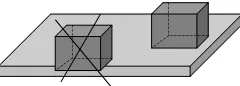
Figure 1: The candidate point is rejected because it does not respect theFace-On-Faceconstraint.
• Candidate point sampling A candidateLc
ikjkis drawn from the distribution
p(Likjk). If we do not have a direct sampling
method from this distribution at our disposal, an indirect sampling method must be used. In this work, we chose to use a Metropolis sampling algorithm [4].
• Candidate validity checking
Suppose we have a geometric relationship be-tween two geometric entitiesEi andEj. A
geo-metrical calculus depending on the type of this relationship allows checking of the constraint
Ck(Qikjk) ≤ 0. If this constraint is respected
(i.e. p(Hk|XikjkLikjk) = 1), the candidateL
c ikjk
is accepted, otherwise it is rejected. Figure 1 shows aFace-On-Facerelationship example.
4.2
Optimization method
For our application, we chose a genetic-based al-gorithm. Since their introduction by Holland [6] in the 1970s, these stochastic techniques have been used for numerous global optimization problems, thanks to their ease of implementation and their independence of application fields [8]. However, practical problems related to the nature of our objective function have to be faced. We propose two major improvements to the genetic algorithm (abbreviated GA) we use.
In the following, we will use G(X) to denote the objective functionp(X|H1· · · HmK1· · · Kp).
4.2.1
Narrowness of the objective
func-tion - constraints relaxafunc-tion
In our applications, the objective function G(X) may have a narrow support (the region where the value is not null) for very constrained problems. The ini-tialization of the population with random individuals from the search space may give null values of the func-tion G(X) for most individuals. This will make the evolution of the algorithm very slow and its behavior will be similar to random exploration.
to first widen the support of the function by changing the original function to obtain non-null values even for configurations that are not permitted. To do so, we introduce an additional parameter we callT (for tem-perature) for the objective function G(X). Our goal is to obtain another functionGT(X) that is smoother
and has wider support, with
lim
T→0G
T(
X) =G(X).
To widen the support ofG(X), all elementary terms (distributions) of this later are widened, namely:
• distributionspOi(Fi(X, L)), wherei= 1· · ·p.
• inequality constraints p(Hm−p+j|Fj(X, L)),
wherej= 1· · ·p.
For example:
• for a Gaussian distribution:
f(x) = √1
2πσe
−12
(x−µ)2
σ2
fT(x) = √ 1
2πσ(1 +T)e
−12
(x−µ)2 [σ(1+T)]2
• for an inequality constraint over the interval [a, b]:
f(x) =
1 if a≤x≤b
0 else
fT(x) =
1 if a≤x≤b
e−
(x−a)2
(b−a)T if x < a
e−
(x−b)2
(b−a)T otherwise
In the general case, inequality constraints may be more complex. Figure 2 shows the case of a Point-On-Face inequality constraint for a square face.
4.2.2
Accuracy of the estimates -
multi-precision computing
The second problem we must face is that only an approximation ˆG(X) ofG(X) is available, of unknown accuracy. Using a large number of points to obtain suf-ficient accuracy may be very expensive in computation time, which makes the use of a large number of points in the whole optimization process inappropriate.
Since the accuracy of the estimate ˆG(X) of the ob-jective function depends on the number N of points used for the estimation, we introduce N as an ad-ditional parameter to define a new function ˆGN(X).
Suppose we initialize and run for some cycles a genetic algorithm with ˆGN1(X) as evaluation function. The
population of this GA is a good initialization for an-other GA having ˆGN2(X) as evaluation function with
N2> N1.
4.2.3
General optimization algorithm
In the following, we label the evaluation function (the objective function) by the temperatureT and the number N of points used for estimation. It will be denoted byGTN(X). Our optimization algorithm may
be described by the following 3 phases.
1. Initialization and initial temperature determina-tion.
2. Reduction of temperature to recreate the origi-nal objective function.
3. Augmentation of the number of points to in-crease the accuracy of the estimates.
Initialization: The population of the GA is initial-ized at random from the search space. To minimize computing time in this initialization phase, we use a small numberN0 of points to estimate integrals. We propose the following algorithm as an automatic ini-tialization procedure for the initial temperature T0, able to adapt to the complexity of the problem.
INITIALIZATION(GA) BEGIN
FOR each population[i]∈GA’s population DO REPEAT
population[i] = random(S) value[i] =GTN
0(population[i])
if (value[i] == 0.0) T = T + ∆T
UNTIL ( value[i]>0.0) FEND
Re-evaluate(population) END
where ∆T is a small increment value.
Temperature reduction: To get the original ob-jective function (T = 0.0), a possible scheduling pro-cedure consists of multiplying the temperature, after running the GA for a given number of cyclesnc1, by a factorα(0< α <1). In this work, the value ofαhas been experimentally fixed to 0.8. We can summarize the proposed algorithm as follows.
TEMP REDUCTION(GA) BEGIN
WHILE (T> T) DO
FOR i=1 TOnc1DO
Run(GA) FEND T = T *α
WEND T = 0.0
Re-evaluate(population) END
whereTis a small threshold value.
Figure 2: The distribution corresponding to inequality constraints induced by aPoint-On-Face relationship for a square face at different values of temperature. The left figure shows the original constraints (T = 0), while the middle and the right ones show these constraints relaxed at (T = 50) and (T = 100) respectively.
To decide between these solutions, we must increase the accuracy of the estimates. One approach is to multiplyN, after running the GA for a given number of cyclesnc2, by a factorβ(β >1) so that the variance of the estimate is divided by β:
V ar(G0β∗N(X)) =
1
βV ar(G
0
N(X)).
We can describe this phase by the following algo-rithm.
N POINTS AUGMENTATION(GA) BEGIN
WHILE (N< Nmax) DO
FOR i=1 TOnc2DO
Run(GA) FEND N = N *β
WEND END
whereNmaxis the number of points that allows convergence of the
estimates ˆG0
N(X) for all individuals of the population.
5
Example
In this section, we describe how to use our CAD system for concrete problems. We present in detail a kinematics inversion problem under geometric uncer-tainties.
5.1
Problem description
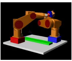
Using two St¨aubli Rx90 robot arms with 6 revo-lute joints, we are interested in placing two prismatic parts one against the other. The only constraint is that a face of the first part will be in a Face-On-Face relationship with a face of the second.
The two arms are modeled as a set of parts attached to each other using probabilistic kinematic links. We assume that the more significant uncertainties are on zero positions. The two parts are also attached to arms’ end effectors using probabilistic kinematic links. The added constraint we wish to satisfy to solve the problem is represented by a link between the two faces
Figure 3: Kinematics inversion example using two St¨aubli Rx90 arms.
TABLE-FACE ARM 1 ARM 2
AXIS 1 2 AXIS 1 1
GRIPPER 1 GRIPPER 2 RED-CUBE BLUE-CUBE FACE 1 FACE 2
Figure 4: The corresponding kinematic graph.
to place in Face-On-Facerelationship. We use for in this link 3 Gaussians on the 3 constrained parameters
tz, rx and ry with zeros as mean values and 0.5mm,
0.01rad and 0.01rad respectively as standard devia-tions. Figure 3 shows the two arms, while Fig. 4 gives the corresponding kinematic graph.
Figure 5: The solution obtained by the system.
Integration space dimension 50 Optimization space dimension 12
Number of cycles 1
Number of frames 28
Number of inequality constraints 16 Computation time (seconds) 13
Table 1: Some parameters summarizing the problem complexity and the system performances for this kine-matics inversion problem.
certainties propagation into account when choosing a solution.
5.2
Results
Figure 5 shows the solution obtained by the sys-tem. This solution gives a maximal precision for the requiredFace-On-Facerelationship because:
1. Arm1 (the less accurate) is coiled to minimize the propagation of the uncertainties on its zero positions.
2. Rotation axes are perpendicular to the common normal of the two faces.
Table 1 summarizes the problem complexity and the system performances for this problem using a Pow-erPC G3/400 machine, while Table 2 gives the state of the cycle we wish to close (the requiredFace-On-Face relationship) after the resolution of the problem.
5.3
Discussion
This example shows how the proposed method takes geometric uncertainties into account in a gen-eral and homogeneous way. No assumptions have been made, either on the uncertainties models (shapes of the used distributions), nor on the linearity of the model or the possibility of it being linearized. It also shows how possible redundancy of the system relating
to the required task is used to find the most accurate solution.
6
Conclusion and Future Research
We have presented a generic approach for geometric problems specification and resolution using a Bayesian framework. We have shown how a given problem is first represented as a kinematic graph, and then for-mulated as an integration/optimization problem. For generality, no assumptions have been made on the shapes of the distributions or on amplitudes of un-certainties.
Experimental results made on our system have demonstrated the effectiveness, the robustness and the homogeneity of representation of our approach. How-ever, additional studies are required to improve both the integration and the optimization algorithms. For the integration problem, numerical integration can be avoided when the integrand is a product of general-ized normals (Dirac’s delta functions and Gaussians) and when the model is linear or can be linearized (er-rors are small enough). The optimization algorithm may also be improved by using a local derivative-based method after the convergence of our genetic algorithm. Future work will aim at allowing the use of high-level sensors such as vision-based ones. We are also consid-ering extending our system so that it can include non-geometrical parameters (inertial parameters for exam-ple) in problem specification.
References
[1] R. Alami and T. Simeon. Planning robust motion strategies for mobile robots. InProc. of the IEEE Int. Conf. on Robotics and Automation, volume 2, pages 1312–1318, San Diego, California, 1994.
[2] Y. Bar-Shalom and T. E. Fortmann. Tracking and Data Association. Academic Press, 1988.
[3] F. Dellaert, D. Fox, W. Burgard, and S. Thrun. Monte Carlo localization for mobile robots. In Proc. of the IEEE Int. Conf. on Robotics and Au-tomation, Detroit, MI, May 1999.
tx(mm) ty(mm) tz(mm) rx(rad) ry(rad) rz(rad)
Mean 5.2070 -71.1645 0.4340 -0.0032 -0.0024 0.2522 Standard deviation 2.8104 5.9147 1.9547 0.0104 0.0143 0.0170
Table 2: The first line gives posterior mean values of the 6 pose parameters of the link to close, while the second line gives standard deviations of this parameters. These values have been obtained empirically using a Monte Carlo simulation with 105sampled points. In bold font, the values of the constrained parameters of the problem, namelytz,rx andry corresponding to the requiredFace-On-Facerelationship.
[5] M. Gondran and M. Minoux. Graphes et Algo-rithmes. Eyrolle, Paris, 1990.
[6] J. H. Holland. Adaptation in Natural and Artifi-cial Systems. University of Michigan Press, Ann Arbor, MI, 1975.
[7] A. Keller. The fast calculation of form factors using low discrepancy point sequence. In Proc. of the 12th Spring Conf. on Computer Graphics, pages 195–204, Bratislava, 1996.
[8] E. Mazer, J.M. Ahuactzin, and P. Bessi`ere. The Ariadne’s Clew algorithm. J. Artif. Intellig. Res. (JAIR), 9:295–316, 1998.
[9] K. Mekhnacha. M´ethodes probabilistes Bayesi-ennes pour la prise en compte des incertitudes g´eom´etriques: application `a la CAO-robotique. Th`ese de doctorat, Inst. Nat. Polytechnique de Grenoble, Grenoble, France, July 1999.
[10] H. P. Moravec. Sensor fusion in certainty grids for mobile robots. AI Magazine, 9(2):61–74, 1988.
[11] J. C. Owen. Constraints on simple geometry in two and three dimensions. Int. J. of Computa-tional Geometry and Applications, 6(4):421–434, 1996.
[12] P. Puget. V´erification-Correction de programme pour la prise en compte des incertitudes en pro-grammation automatique des robots. Th`ese de doctorat, Inst. Nat. Polytechnique de Grenoble, Grenoble, France, 1989.
[13] A. C. Sanderson. Assemblability based on max-imum likelihood configuration of tolerances. In Proc. of the IEEE Symposium on Assembly and Task Planning, Marina del Rey, CA., August 1997.
[14] R.H. Taylor. A synthesis of manipulator control programs from task-level specifications. Ph.d the-sis, Stanford University, Computer Science De-partment, July 1976.