Determination Of A Nonresidential Space Cooling Load: Vb Program Apprication

(1)

Determination Of A Nonresidential Space Cooling

Load: Vb Program Apprication

Obuka, Nnaemeka S.P., Utazi, Divine N., Onyechi, Pius C., Okoli, Ndubuisi C., Eneh, Collins O.

ABSTRACT:This study develops a computer application in Visual Basic computer programming language capable of computing the sensible and latent cooling loads of a single zone of a non-residential building taking all the influential factors into consideration, using the CLTD/SCL/CLF method.The developed program is enhanced with a special Graphical User Interface (GUI) to make it more User friendly. Basic equations relating to the problem were presented, these are mainly assumptions proposed by ASHRAE for its calculation of heat gain and cooling load.The calculation was based on the atmospheric condition and parameters obtainable in the month of March at 8hours interval between the 8.00hrs and 16.00hrs of the day. This space cooling load calculation was carried out for an actual building in University of Nigeria Nsukka (i.e. 3rd year lecture room in Mechanical Engineering Department) using the developed program and the maximum space loads which are required for the space are 11432 watts sensible and 4120 watts latent.

KEYWORDS: Visual Basic, Cooling Load, CLTD/SCL/CLF Method, Graphical User Interface, Heat gain

————————————————————

1 INTRODUCTION

In tropical and subtropical countries, cooling by means of air-conditioning is a necessary feature of modern development as the new and emerging industries and households need it to retain reliability of some industrial and home based appliances. Air-conditioning system is designed with ability to subdue most common heat loads such as sensible and latent heat [1], [2].Cooling load calculations are carried out to estimate the required capacity of cooling systems, which can maintain the required conditions in the conditioned space.For estimating cooling loads, one has to consider the unsteady state processes, as the peak cooling load occurs during the day time and the outside conditions also vary significantly throughout the day due to solar radiation. In addition, all internal sources add on to the cooling loads and neglecting them would lead to underestimation of the required cooling capacity and the possibility of not being able to maintain the required indoor conditions. Thus cooling load calculations are inherently more complicated as it involves solving unsteady equations with unsteady boundary conditions and internal heat sources.The total building cooling load consists of heat transferred through the building envelope (walls, roof, floor, windows, doors etc.) and heat generated by occupants, equipment, and lights.

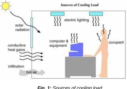
The load due to heat transfer through the envelope is regarded as ‗external load‘, while all other loads are referred to as ‗internal loads‘.The percentage of external versus internal load varies with building type, site climate, and building design. The total cooling load on any building consists of both sensibleas well as latentload components. The sensible load affects dry bulb temperature, while the latent load affects the moisture content of the conditioned space.The heat transfer due to ventilation is not a load on the building but a load on the system. The various internal loads consist of sensible and latent heat transfer due to occupants, products, processes and appliances, sensible heat transfer due to lighting and other equipment. Fig. 1, shows various components that constitute the cooling load on a building.

1.1 Space Characteristics and Heat Load Sources. In estimating the the heat load the following physical aspects are worth considering: (a) Orientation of the building: This aspect defines the location of the conditioned space with respect to (i) Compass points for sun and wind effects (ii) the adjoining permanent structures for shading effects. (b) Use of conditioned space. It may be used for office, or hospital, or some shop, residence. (c) Physical dimension of spaces: Length, width and height are recorded. (d) Ceiling height: Floor-to-floor height or floor to ceiling height may be noted down. (e) Construction materials: The materials of construction used, thickness of walls and roofs, floors and partitions and their location in the building structure are noted. (f) Windows: Size and

Fig. 1: Sources of cooling load

___________________________

 Obuka, Nnaemeka S.P., Utazi, Divine N., Onyechi,

Pius C., Okoli, Ndubuisi C., Eneh, Collins O.

 Department of Mechanical/production Engineering,

Enugu State University of Science and Technology, Enugu, Nigeria.

 Department of Mechanical Engineering, University of

Nigeria, Nsukka, Nigeria.

 Department of Industrial and Production

Engineering, Nnamdi Azikiwe University, Awka, Nigeria.

(2)

location of windows, the type of glass used and whether single or double double is to be noted. Also the type of shading on it must be noted. (g) People: The number of people, their duration of occupancy, their nature of work activity and any special features like concentration at any place in the conditioned space must be noted. (h) Lighting: The load in watts at peak, the nature of load incandescent, florescent must be noted. (i) Appliances: Location, rated wattage for the appliances must be considered. (j) Continuous and intermittent operation: Whether the plant has to operate every day of the season or only occasionally as in churches and ballrooms.

2. LITERATURE

ON

THE

EVOLUTION

OF

COOLING

LOAD

CALCULATION

METHODS

The method for peak cooling load calculation dated as early as 1894 [3]. However, during the period prior to 1945, there were best inconsistent methods for calculating peak heating and cooling loads, nevertheless, the foundation was laid for today‘s modern methods, which began with sol-air temperatures, decrement factors and the use of a thermal R/C network. Most of the dynamic peak cooling calculation methods used today were proposed during the 1946-1969 period. Stewarts [4] outlined the Equivalent Temperature Differentials (ETD) based on Mackey and Wright‘s earlier work. The ETD tables were adopted by American Society of Heating and Ventilating Engineers (ASHVE) Guide in 1951 [5], but due to its shortfalls additional tables of Total Equivalent Temperature Difference/Time Averaging (TETD/TA) method values were tabulated in the 1961 ASHRAE Guide and Data Book [6]. Gay et al [7] in their book included a revised procedure for air conditioning design, as well as improved data for calculating heat gains. Brisken et al [8], laid the foundation of today‘s thermal Response Factor Method (RFM) based on Nessi and Nisolle‘s 1925 work. Based on the work of Brisken et al, Mitalas and Stephenson [9] developed the thermal response factor method which allowed for solution to the dynamic heat transfer problem without having the knowledge of how to solve separate differential equation for each new wall type. This method became part of the Weighing Factor Method (WFM), which was used in the 1981 ASHRAE Hand book [10]. The Finite Difference/Finite Element Method (FDM/FEM) was introduced in 1960 [11], [12] in the form of formal equations that could be directly used in computer algorithms. The admittance method was developed by Loudon [13], while the concept of Thermal Admittance was first introduced in U.K by the Institute of Heating and Ventilating Engineers (IHVE) Guide in 1970 [14]. The ASHRAE Task Group on Energy Requirements (TGER) first introduced the Transfer Function Method (TFM), which was based on Mitalas and Stephenson‘s earlier work and it is considered the first, wide spreadcomputer oriented method for solving dynamic heat transfer problems in buildings [15]. Rudoy and Duran [16] developed the Cooling Load Temperature Difference/Cooling Load Factor (CLTD/CLF) method, which included tabulated results of controlled variable tests summarized in ASHRAE research project RP-138. The CLTD/CLF method attempted to simplify the two-step TFM and TETD/TA method into a single-step technique published in the 1977 ASHRAE Handbook of Fundamentals [17]. However, the CLTD/CLF method was modified by Prof.

Edward Sowell, who ran 200,640 simulations to provide new tabulated answers [18]. Harries and McQuiston [19] proposed an additional Conduction Transfer Function (CTF) coefficients to cover more groups of roof and wall construction conditions. Spitler et al [20] updated the CLTD/CLF method to become the CLTD/SCL/CLF method by introducing the term Solar Cooling Load (SCL) for an improved solar heat gain calculation through fenestration. The most current cooling load calculation method is the Radiant Time Series (RTS) method which is an improvement over all previous methods [21]. The accuracy of the RTS method is similar to that of TFM if custom weighing factors and custom conduction transfer function coefficient were used for all components in a building. ASHRAE building load calculation toolkit (LOAD toolkits) was developed by Pedersen et al [22] which provided a FORTRAN source code for peak heating/cooling calculations for ASHRAE members to use. Finally, for residential load calculations, the Residential Heat Balance (RHB) and the Residential Load Factor (RLF) methods were developed to be a computer algorithm coded using FORTRAN [23].

2.1 Computer Application in Cooling Load Calculation:

(3)

3. MATERIALS

AND

APPLICABLE

METHOD

This work was carried out to calculate a non-residential cooling and heating load capacity through the application of the CLRD/SCL/CLF method using a computer program with the Visual Basic (VB) programming language. The CLTD/SCL/CLF method is a one-step, hand calculation procedure based on the Transfer Function Method (TFM). It may be used to approximate the cooling load corresponding to the first three modes of heat gain (conductive heat gain through surfaces such as windows, walls, and roofs; solar heat gain through fenestration; and internal heat gain from light, people, and equipments) and the cooling load from infiltration and ventilation [25]. This method as with any method requires engineering judgement in its application. When the method is used in conjuction with custom tables generated by appropriate computer software [26] and for buildings where external shading is not significant, it can be expected to produce results very close to those produced by the TFM.

3.1 Space Design Cooling Load Calculation by CLTD/SCL/CLF

3.1.1 External Cooling Loads:

(i) Roofs, walls and glass: The basic cooling load equation for exterior surfaces such as roofs, walls, and conduction through glass is given as;

q = U × A × CLTD (1)

Where: q is cooling load, W; U is coefficient of heat transfer, W/(m2k) (Chapter 24 of [27]); A is area of surface, m2; CLTD is cooling load temperature difference, roof, wall or glass.

(ii) Fenestration: Space cooling load from fenestration include the heat gain from conduction and solar radiation. The cooling load from conduction and convection heat gain is calculated by;

qcond = U × A × (CLTD) (2)

Where: qcond is cooling load caused by conduction and convection, W; A is net glass area of the fenestration, m2. While the cooling load caused by solar radiation through fenestration is calculated by;

qrad = A × SC × SCL (3)

Where: qrad is cooling load caused by radiation, W; A is net glass area of fenestration, m2; SC is shading coefficient for combination of fenestration and shading device (Chapter 29 of [27]); SCL is solar cooling load, W/m2 (Table 36 of [27]). Therefore, the total cooling load due to fenestration is the sum of the conductive and radiant components qcond and qrad.

(iii) Partitions, ceilings, and floors: The cooling load from partitions, ceilings, and floors is calculated as follows;

q = U × A ta− trc (4)

Where: U is design heat transfer coefficient for partition,

ceiling or floor (Chapter 24 of [27]); A is area of partition, ceiling or floor calculated from building plans; ta is temperature in adjacent space; trc is inside design temperature (constant) in conditioned space.

3.1.2 Internal Cooling Loads:

(i) People: The total sensible heat gain from people is not converted directly to cooling load. The radiant portion is first absorbed by the surroundings (floor, ceiling, partition, furniture) then convected to the space at a later time, depending on the thermal characteristics of the room. Hence, the instantaneous sensible cooling load due to people is calculated thus;

q_s= N × SHG_p CLF_p (5)

And the latent cooling load due to people is:

q_l= N × LHG_p (6)

Where: qs is sensible cooling load due to people; N is number of people; SHGp is sensible heat gain per person (Chapter 8, ASHRAE 1997); CLFp is cooling load factor for people (Table 37, ASHRAE 1997); ql is latent cooling load due to people; LHGp is latent heat gain per person (Chapter 8 of [27]).

(ii) Lights: At any time, the space cooling load from lighting can be estimated as;

qel = W × Ful× Fsa× CLFel (7)

Where: W is watts input from electrical plans or lighting fixture data; Ful is lighting use factor as appropriate; Fsa is special allowance factor as appropriate; CLFel is cooling load factor for lights (Table 38, ASHRAE 1997).

(iii) Power: The cooling load value of power-driven equipments can be calculated as:

q_p= P × E_f× CLF (8)

Where: P is horsepower rating from electrical plans or manufacturer‘s data; Ef is efficiency factors and arrangements to suit circumstances; CLF is cooling load factor by hour of occupancy (Table 37 of [27]).

(iv) Appliances: To calculate the cooling load capacity of appliances in a particular circumstance either of the following equations can be applied;

qsensible = qinput × FU× FR× CLF (9)

Or,

q_sensible = q_input × F_L× CLF (10)

(4)

3.1.3 Ventilation and Infiltration Air: Space cooling load due to ventilation and infiltration air is calculated as follows;

qsensible = 1.23 × Q to− ti (11)

qlatent = 3010 × Q W0− Wi (12)

qtotal = 1.20 × Q h0− hi (13)

Where: Q is ventilation from ASHRAE standard 62; t0, ti are outside and inside air temperatures, 0C; W0. Wi are outside and inside air humidity ratio, kg (water), kg (dry air); h0, hi are outside and inside air enthalpy, k/kg (dry air).

3.2 The Computer Program:

In the previous subsection various formulae and methods, for calculating hourly cooling load of a building, are discussed in detail. To make the computation friendly and time effective a computer program is developed using

Visual Basic Programming Language.The program developed can be broadly classified as follows: (a) Program for calculating heat gain through wall and roof. (b) Program for calculating heat gain through window or glass. (c) Program for calculating heat gain through infiltration. (d) Program for calculating internal heat gain. (e) Program for calculating space cooling load from heat gain. To make the programs developed a user-friendly type, GUI (graphic user interface) is developed. So any person with out knowing the detail of the program can run and have the hourly cooling load of the building.

3.2.1 Development of the GUI: There are fifteen GUI programs developed. The first program ―starting window‘‘, Fig. 1 is used to display the title of the thesis. Besides this feature it has one push button, ‗Next‘, the button leads to the remaining parts of the program. If the user selects ‗Next‘ button, the module will be automatically shifted to the next part, input module, Fig. 2.

This module enables the user to enter the values of design room temperature, design outdoor temperature, length of the space, etc. This module has four push buttons ‗Reset‘, ‗Skip‘, ‗Next‘ and ‗Exit‘. The ‗Reset‘ button clears the entered values, ‗Skip‘ button skips the load source calculation and shift the program to roof load source module, ‗Exit‘ button helps to terminate the program and If

the user selects ‗Next‘ button after entering the values, a module for roof load source, Fig. 3, appears. This module enables the user to choose roof type, solar time, month and latitude of the location. There are also four push buttons, Back, Skip, Next and Exit with functions similar to their name.

Fig. 1: Starting window Fig. 2: Inputs window

(5)

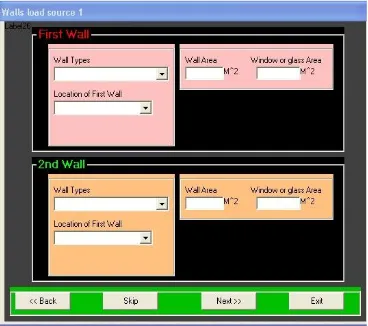
The walls load source 1 module, Fig. 4, appears when the user selects ‗Next‘ button in the input window module. This module enables the user to selects and enters values such

as wall type, wall location, wall area, etc for first and second walls of the building. The other three push buttons, Back, Skip, and Exit functions similar to their name.

The walls load source 2 module, Fig. 5, appears when the user selects ‗Next‘ button in the wall load source 1 module. This module enables the user to selects and enters values such as wall type, wall location, wall area, etc for third and fourth walls of the building. The other three push buttons, Back, Skip, and Exit functions similar to their name. The module ―choose wall with glass‖, Fig. 6, which appears

when the user selects ‗Next‘ or ‗Skip‖ button in the wall load source 2 module, composed of four input modules for load through glass. The first module, Fig. 7, will appear when the user selects ‗1‘ from combo box ‗How many of the walls has window or glass on it‘ and click on ‗Next‘ button. When ‗2‘ is selected, the modules Fig. 7 and Fig. 8 will appear consecutively when the ‗Next‘ buttons are selected.

Fig. 5: Wall load source 2 Fig. 6: Choose wall with glass

Fig. 7: First window or glass load source. Fig.8:2nd window or glass load source.

(6)

When ‗3‘ is selected, the modules Fig. 7; Fig. 8 and Fig. 9 will appear consecutively when the ‗Next‘ buttons are selected. While the modules Fig.7, Fig. 8, Fig. 9 and Fig. 10 will appear consecutively when ‗4‘ is selected. If the user

selects ‗Skip‘ button, the module load source will not be calculated and automatically shifted to the next part, internal load source module, Fig. 11.

This module enables the user to selects the lamp type and enter the value of lamp capacity. This module has four push buttons ‗Back‘, ‗Skip‘, ‗Next‘ and ‗Exit‘. If the user selects ‗Next‘ button, a module for people load source, Fig. 12, appears. This module enables the user to select people‘s degree of activity in the building. The appliances load

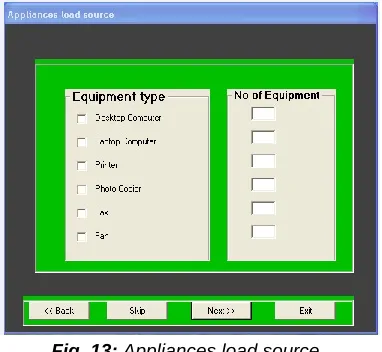
source module, Fig. 13, appears when the user selects ‗Next‘ button in the internal light load source module. This module enables the user to selects equipment type and it‘s no in a room. The other three push buttons, Back, Skip, and Exit functions similar to their name.

The infiltration load source module, Fig. 14, appears when the user selects ‗Next‘ button in the appliances load source module. This module enables the user to selects space construction and pressurization. The other three push buttons, Back, Skip, and Exit functions similar to their name. Finally, the space cooling load summary module, Fig. 15, appears when the user selects ‗Next‘ button in the infiltration load source module. This module displays the calculated values of sensible and latent loads of different load source.The push buttons, ‗Back‘ and ‗Exit‘ functions similar to their name.

Fig. 11: Internal light load source Fig. 12: People load source

Fig. 13: Appliances load source Fig. 14: Infiltration load source.

(7)

4. RESULT

AND

DISCUSSION

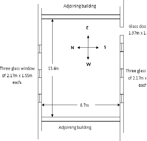
This developed program was used to calculate the space cooling load of a 3rd year classroom of Mechanical Engineering Department in University of Nigeria Nsukka. The plan of the classroom is shown in Fig. 16.

TABLE 1:MEASURED PARAMETERS

Wall construction Floor- to- ceiling height Roof type

Window and Door Lights

Occupancy Appliances Working duration

8-in. (0.203m) concrete block (U=2.283 W/m2-0C) 3.9m

Pitched roof (U = 0.801 W/m2-0C)

Single glass without shade (U=5.906 W/m2-0C) Four fluorescent tubes of 36 watts each

70 persons

5 Laptop computers 8 hours (8.00am – 4.00pm)

TABLE 2:DESIGN CONDITIONS

Month Location

Room design dry-bulb Outdoor design dry-bulb Daily temperature range Relative humidity

Design indoor humidity ratio Design outdoor humidity ratio Space construction and presurisation

March 80N latitude 25.60C 350C 190C 50%

0.010kg/kg of air 0.018kg/kg of air

Pressurized, Average construction

Through the application of Visual Basic programming language the computer algorithms and commands were developed based on the applicable equations as stated in equations (1) to (13), then the above given parameters and

design conditions are computered into the program with the help of the developed GUI. At this juncture the following result (Table 3) was obtained from the computer program.

(8)

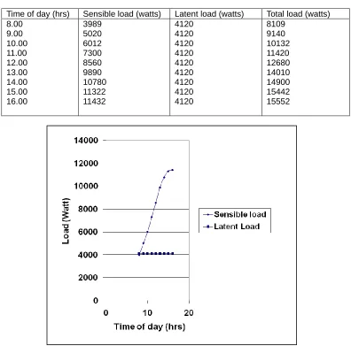
TABLE 3:THE RESULT OBTAINED FROM THE DEVELOPED PROGRAM

Time of day (hrs) Sensible load (watts) Latent load (watts) Total load (watts) 8.00

9.00 10.00 11.00 12.00 13.00 14.00 15.00 16.00

3989 5020 6012 7300 8560 9890 10780 11322 11432

4120 4120 4120 4120 4120 4120 4120 4120 4120

8109 9140 10132 11420 12680 14010 14900 15442 15552

From the sensible load graph above, sensible load increases with the time of the day. This shows that the more the exterior of the space is been heated by the sun, the more the heat that is conducted and trasmmited to the space, the more the sensible load increase.While the latent load graph remains the same with the increase in the time of the day. This is because the components of the latent load here are latent heat gain from infiltration and latent heat gain from people within the space, and it‘s constant for each time of the day.

5. CONCLUSION

Theprogram can be used for cooling load estimation of other single zone structures like Auditorium and offices, provided that the dimensions are well determined.The space cooling load of an actual building in University of Nigeria Nsukka (i.e. 3rd year classroom in Mechanical Engineering Department) is computed using the developed program.The maximum space loads which are required for the space are 11432 watts sensible and 4120 watts latent.The same result was obtained when space cooling load is manually calculated using CLTD/SCL/CLF method. Traditionally, load estimating for air conditioning systems is done either by manual calculation or judgmental estimation

based on experience of the air conditioning practitioner. This program will help to reduce the laborious nature of manual calculation and liable errors due to judgmental estimation.

REFERENCES

[1] Adeyemo, T. (2000). Refrigeration and the Air Conditioning, GreenlinePublishers, Nigeria, pp 113.

[2] James, C.W., (1995). Air Conditioning Technology,Wellington Publishers, USA. pp 413.

[3] Harberl, J.S., and Baltazar, J. (2013). Literature Review on the History of Building Peak Load and Annual Energy Use Calculation Methods in the U.S. Energy Systems Laboratory, Texas A&M University, Texas, U.S.A.

[4] Stewart, J.P. (1948). Solar Heat Gain through Walls and Roofs for Cooling Laod Calculations. ASHVE Transaction 54, pp 361-389.

[5] ASHVE. (1951). American Society of Heating and Ventilating Engineers Guide. American Society of

(9)

Heating and Ventilating Engineers, New York, U.S.A.

[6] ASHRAE. (1961). ASHRAE Guide and Data Book 1961: Fundamentals and Equipment. American Society of Heating, Refrigerating and Air-Conditioning Engineers, New York.

[7] Gay, C.M., Fawcett, C.D.V., and McGuinness, W.J. (1955). Mechanical and Electrical Equipments for Buildings. (3rd ed.). John Wiley and Sons, New York.

[8] Brisken, W.R., and Reque, S.G. (1956). Heat Loading Calculations by Thermal Response. ASHRAE Transactions, 62, pp 391-424.

[9] Mitalas, G.P., and Stephenson, D.G. (1967). Room Thermal Response Factor. ASHRAE Transactions, 73. Pt. 1.

[10]ASHRAE. (1981). ASHRAE Handbook: 1981 Fundamentals. American Society of Heating, Refrigerating and Air-Conditioning Engineers, Atlanta-Georgia, U.S.A.

[11]Clough, R.W. (1960). The Finite Element Method in Plain Stress Analysis. Proceedings of Second ASCE Conference on Electronic Computation, Pittsburg, Pennsylvania, Vol. 8, pp 345-378.

[12]Forsythe, G.E., and Wasow, W.R. (1960). Finite Difference Methods for Partial Differential Equations. John Wiley ans Sons Inc., New York, NY.

[13]Loudon, A.G. (1968). Summertime Temperatures in Building without Air-Conditioning. Building Research Station, Report No. BRS-CP-47-68.

[14]Goulert, S.V.G. (2004). Thermal Inertia and Natural Ventilation – Optimization of Thermal Storage as a Cooling Technique for Residential Biuldings in Southern Brazil. Ph.D Dissertation, Architectural Association School of Architecture Graduate School, the Open University.

[15]Mitalas, G.P. (1972). Transfer Function Method of Calculating Cooling Loads, Heat Extraction and Space Temperature. ASHRAE Journal, Vol. 14, Issue 12, pp 54-56.

[16]Rudoy, W., and Duran, F. (1974). Development of an Improved Cooling Load Calculation Method Final Report. American Society of Heating, Refrigerating and Air-Conditioning Engineers, ASHRAE-RP-138, Atlanta Georgia, U.S.A.

[17]ASHRAE. (1977). ASHRAE Handbook of Fundamentals. American Society of Heating, refrigerating and Air-Conditioning Engineers, Inc.,

New York, NY.

[18]Sowell, E.F. (1988). Classification of 200,640 Parametric Zones for Cooling Load Calculation. ASHRAE Transactions, Vol. 94, Pt. 2, pp 754-777.

[19]Harries, S.M., and McQuiston, F.C. (1988). A Study to Catagorize Walls and Roofs on the Basis of Thermal Response. ASHRAE Transactions, Vol. 94, Pt 2, pp 688-715.

[20]Spitler, J.D., McQuiston, F.C., and Lindsey, K.L. (1993). The CLTD/SCL/CLF Coolindg Load Calculation Method. ASHRAE Transaction, Vol. 99, No. 1, pp 183-192.

[21]Spitler, J.D., Fisher, D.E., and Pedersen, C.O. (1997). The Radiant Time Series Cooling Load Calculation Procedure. ASHRAE Transactions, Vol. 103, Pt. 2, pp 503-515.

[22]Pedersen, C.O., Fisher, D.E., Liesen, R.J., and Strand, R.K. (2003). ASHRAE Toolkit for Building Load Calculation. ASHRAE Transactions, Vol. 109, Pt. 1, pp 583-589.

[23]Barnaby, C.S., Spitler, J.D., and Xiao, D. (2004). Updating the ASHRAE/ACCA Residential Heating and Cooling Load Calculation Procedures and Data.ASHRAE Final Report 1199. American Society of Heating, Refrigerating and Air-Conditioning Engineers, Inc., Atlanta, Georgia.

[24]Fantu, K. (2004). Transint Analysis of Cooling Load of a Single Zone Building. M.Sc. Thesis, Mechanical Engineering Department, School of Graduate Studies, Addis Ababa University.

[25]ASHRAE. (2001). ASHRAE Handbook Fundamentals. American Society of Heating, Refrigerating and Air-Conditioning Engineers, Inc., Atlanta, Georgia, U.S.A.

[26]McQuiston, F.C., and Spitler, J.D. (1992). Coolind and Heating Load Calculation Manual. 2nd ed. ASHRAE.