Introduction to Physical Oceanography

(1)

PHYSICAL OCEANOGRAPHY

Introduction to

Robert H Stewart

(2)

Introduction to Physical Oceanography

Robert Stewart

Texas A&M University

Copyright

I hereby grant any user right to download and print a copy of the book for personal use. I also grant all teachers, lecturers, and professors the right to download the book and to make multiple copies for use by their students. The multiple copies may be made by copy centers. Students may be charged the cost of reproducing the book.

I do not grant rights to the text for commercial purposes. Download the Book

These files are the latest version, August 13, 2008. The files are in Adobe Portable Document Format. This version has hyperlinked Table of Contents and Index for easier navigation of the document in Adobe Acrobat Reader. I thanks Andrew Kiss of the University of New South Wales in Canberra Australia for his help in using the \hyperref package to produce the links.

Book Complete book in a 9.6 Mbyte file with index.

Cover Color cover for your book.

If you don't have an Acrobat Reader, you can download one for free from Adobe. Introduction

This is a new textbook describing physical-oceanographic processes, theories, data, and measurements. In addition to the classical topics, I have included discussions of heat fluxes, the role of the ocean in climate, the deep circulation, equatorial processes including El Nino, data bases used by oceanographers, the role of satellites and data from space, ship-based measurements, and the importance of vorticity in understanding oceanic flows.

I have used the text to teach upper-division undergraduates and graduate students in oceanography, meteorology, and ocean engineering. Because many students have already taken courses that emphasize math, I have minimized the math and emphasized processes. Still, students should have studied differential equations and introductory college physics. The text is typeset and it has high-resolution figures produced by Adobe Illustrator CS2. The book was produced in LATEX2ε using TeXShop 2.14 on an Intel dual-processor iMac running OS-X 10.4.11. The resulting typeset, 345 page, book.pdf file is only 9.5 Megabytes. If you make multiple copies I recommend you use a copy center that can make copies directly from the book.pdf file. These copies will be much better than copies made from printed pages.

If you have problems, please contact me at [email protected]

Web Version

A web-based version the book is also available..

What's New!! Fall 2008 Revisions

This edition has a few minor and more important changes:

Corrected a few minor errors. There are less and less thanks to the many readers who have found errors in the 1.

Book PDF Files http://oceanworld.tamu.edu/resources/ocng_textbook/PDF_files...

(3)

past.

Added information about the new Reference Salinity scale in Section 6.1. 2.

Corrected an important error in my discussion of potential temperature in Section 6.5. 3.

Added information about MODIS and Jason-2. 4.

Removed references to controversy about vertical mixing in the ocean in Section 8.4. The controversy has been resolved.

5.

Added more information about abrupt climate at end of the last ice age in Section 13.1. 6.

Added more information about mixing driving the deep circulation in Section 13.3 and , and the role of Ekman pumping in the Antarctic and its influence on the deep circulation in Section 13.5

7.

Added information about measured variability of the North Atlantic meridional overturning circulation in Section 13.4. 8.

Removed information about solitons in Section 16.2. It is not that important in an introductory text that is alreay too long.

9.

The table below links to the latest version of Introduction to Physical Oceanography in Adobe Acrobat Portable Document Format (pdf files). The files may be downloaded and printed if you wish a nice printed copy of the book. Altogether, there are viii + 345 pages in the book.

Fall 2007 Revisions

This edition has several changes from the previous edition. The changes include:

Mostly many small changes and corrections of minor errors. I thank all of you who have emailed comments to me this year.

1.

COADS has been changed to the new ICOADS. 2.

Revised section on definition of salinity to separate definition from extensions of definition to typical temperatures found in the ocean.

3.

Revised section on temperature to refer to the new Smith and Reynolds Improved Optimal Interpolation scheme. 4.

Added information on Prandtl's discovery of the boundary layer and its importance to oceanography 5.

Revised paragraphs on altimeter errors to include more accurate values now being achieved for Jasin and Topex/Poseidon.

6.

Revised figure 12.7 to show western intensification. 7.

Clarified importance of equatorial heating for atmospheric circulation, and role of el Nino. 8.

Added information on the Advanced Circulation Model for coastal processes and storm surges. 9.

This edition has several changes from the previous edition. The changes include:

Updated information on maps of seafloor features and global bathymetric maps. 1.

Revised section on measurements of winds to better describe satellite measurements of winds. 2.

Revised section on measurements of currents to state more clearly the important techniques and drop less important information.

3.

Dropped the description of fresh-water transports. I think the topic is beyond the scope of the book. 4.

Made a few minor changes in wording and corrected a very small number of typographical errors. I thank all of you who have found almost all errors in previous years.

5.

As a result, the book is one page shorter this year. 6.

The files below are the latest version, August 10, 2005.

This edition has only minor changes from the previous edition. The changes include:

Clarified the discussion of important forces in Chapter 7. 1.

Dropped all statements that a derivation is simple. It may be simple to some, but not to many students. 2.

Added a new figure on Ekman flow in Chapter 9. 3.

Revised the discussion of flow into and out of the Mediterranean Sea in Chapter 7. 4.

(4)

Made a few minor changes in wording and corrected a few typographical errors. 5.

Deleted all references to the practical salinity unit (psu). It doesn't exist. Salinity is a dimensionless ratio of masses. 1.

Clarified the derivation of Margules' equation on page 171. 2.

Spring 2004 Revisions

Revision of discussion of using vorticity to explain western boundary currents on page 204-205. 1.

Changed explanation of tide generating forces on page 301. 2.

Corrected error in equations describing the Ekman layer on page 139. 3.

Corrected errors in figure 3.2. 4.

Clarified differences between a surface analysis and reanalyzed weather data on pages 47. 5.

The important changes include:

Many figures have been redrawn, some have been replaced. 1.

The index is much improved. 2.

Many references have been deleted or added. The calls to references in the text now agree with references at the end of the book.

3.

Chapter 13 on the deep circulation has been revised to include recent advances in our understanding of the deep mass flow. Out is any reference to the thermohaline circulation (it is used in too many conflicting ways). In is the information that the deep flow is driven by wind and tidal mixing.

4.

Hundreds of minor revisions throughout the book. 5.

We have an index! Trey Morris, a student, spent the summer tagging all the LaTeX files used to make the book. From these we produced an index and the pdf files below.

1.

Don Johnson, another student, spent months redrawing many figures. 2.

I simplified some of the discussions of errors. I found that students jumped to the conclusion that if there were several sources of error, no matter how small, the data were essentially worthless. This shortened the book by seven pages.

3.

I made hundreds of small changes to the text. 4.

Spring 2002 Revisions

Gradually replacing poor scanned images with newly redrawn figures. 1.

Corrected some significant errors in Chapter 10: tables had wrong values in one column, and text describing how currents are calculated from measurements of density was confusing

2.

Many minor changes in all chapters. 3.

The book is one page longer. 4.

Adobe index file added. 5.

(5)

A beautiful cover. 1.

Clarified the values for vertical diffusivity removing the conflict between Munk's value and measurements. 2.

Revised the discussion of Ekman pumping and the role of vorticity in section 12.3. 3.

Revised section 6.5 on density. 4.

Added a description of neutral density. 5.

Revised or redrew many figures. 6.

Corrected many, many typos and other minor irritating errors. 7.

The book is a few pages shorter. 8.

Plus, I learned more about Adobe Illustrator 9 and Distiller 5 than I ever wanted to know. My testing leads me to believe the pdf files will print correctly.

9.

I have revised many sections of the book, added new figures illustrating key concepts, and corrected many small errors. The important changes include:

More information on double diffusion. 1.

Much revised section on Ekman currents. 2.

Added description of the North Atlantic circulation in chapter 10, including discussion of the Gulf Stream and negative viscosity.

3.

Clarified that vertical mixing drives the deep circulation, and added a description of the Antarctic Circumpolar Current in Chapter 13.

4.

Revised discussion of El Nino/La Nina. 5.

Dropped the old Chapter 15 on the observed circulation of the ocean and added the information to other chapters. 6.

Department of Oceanography, Texas A&M University Robert H. Stewart, [email protected]

URL: http://oceanworld.tamu.edu/resources/ocng_textbook/PDF_files/book_PDF_files.html

(6)

Introduction To

Physical Oceanography

Robert H. Stewart Department of Oceanography

Texas A & M University

(7)

(8)

Preface

This book is written for upper-division undergraduates and new graduate dents in meteorology, ocean engineering, and oceanography. Because these stu-dents have a diverse background, I have emphasized ideas and concepts more than mathematical derivations.

Unlike most books, I am distributing this book for free in digital format via the world-wide web. I am doing this for two reasons:

1. Textbooks are usually out of date by the time they are published, usually a year or two after the author finishes writing the book. Randol Larson, writing in Syllabus, states: “In my opinion, technology textbooks are a waste of natural resources. They’re out of date the moment they are published. Because of their short shelf life, students don’t even want to hold on to them”—(Larson, 2002). By publishing in electronic form, I can make revisions every year, keeping the book current.

2. Many students, especially in less-developed countries cannot aﬀord the high cost of textbooks from the developed world. This then is a gift from the US National Aeronautics and Space Administrationnasato the students of the world.

Acknowledgements

I have taught from the book for several years, and I thank the many students in my classes and throughout the world who have pointed out poorly written sections, ambiguous text, conflicting notation, and other errors. I also thank Professor Fred Schlemmer at Texas A&M Galveston who, after using the book for his classes, has provided extensive comments about the material.

I also wish to thank many colleagues for providing figures, comments, and helpful information. I especially wish to thank Aanderaa Instruments, Bill Al-lison, Kevin Bartlett, James Berger, Gerben de Boer, Daniel Bourgault, Don Chambers, Greg Crawford, Thierry De Mees, Richard Eanes, Peter Etnoyer, Tal Ezer, Gregg Foti, Nevin S. Fuˇckar, Luiz Alexandre de Araujo Guerra, Hazel Jenkins, Jody Klymak, Judith Lean, Christian LeProvost, Brooks Martner, Nikolai Maximenko, Kevin McKone, Mike McPhaden, Thierry De Mees, Pim van Meurs, Gary Mitchum, Joe Murtagh, Peter Niiler, Nuno Nunes, Ismael N´u˜nez-Riboni, Alex Orsi, Kym Perkin, Mark Powell, Richard Ray, Joachim Ribbe, Will Sager, David Sandwell, Sea-Bird Electronics, Achim Stoessel, David

(13)

viii PREFACE

Stooksbury, Tom Whitworth, Carl Wunsch and many others.

Of course, I accept responsibility for all mistakes in the book. Please send me your comments and suggestions for improvement.

Figures in the book came from many sources. I particularly wish to thank Link Ji for many global maps, and colleagues at the University of Texas Center for Space Research. Don Johnson redrew many figures and turned sketches into figures. Trey Morris tagged the words used in the index.

I especially thanknasa’s Jet Propulsion Laboratory and the Topex/Poseidon and Jason Projects for their support of the book through contracts 960887 and 1205046.

Cover photograph of the resort island of Kurumba in North Male Atoll in the Maldives was taken by Jagdish Agara (copyright Corbis). Cover design is by Don Johnson.

The book was produced in LA_{TEX 2}_ε _{using TeXShop 2.14 on an Intel iMac}

(14)

Chapter 1 A Voyage of Discovery

The role of the ocean on weather and climate is often discussed in the news. Who has not heard of El Ni˜no and changing weather patterns, the Atlantic hurricane season and storm surges? Yet, what exactly is the role of the ocean? And, why do we care?

1.1 Why study the Physics of the ocean?

The answer depends on our interests, which devolve from our use of the ocean. Three broad themes are important:

1. We get food from the ocean. Hence we may be interested in processes which influence the sea just as farmers are interested in the weather and climate. The ocean not only has weather such as temperature changes and currents, but the oceanic weather fertilizes the sea. The atmospheric weather seldom fertilizes fields except for the small amount of nitrogen fixed by lightning.

2. We use the ocean. We build structures on the shore or just oﬀshore. We use the ocean for transport. We obtain oil and gas below the ocean. And, we use the ocean for recreation, swimming, boating, fishing, surfing, and diving. Hence we are interested in processes that influence these activities, especially waves, winds, currents, and temperature.

3. The ocean influence the atmospheric weather and climate. The ocean influence the distribution of rainfall, droughts, floods, regional climate, and the development of storms, hurricanes, and typhoons. Hence we are interested in air-sea interactions, especially the fluxes of heat and water across the sea surface, the transport of heat by the ocean, and the influence of the ocean on climate and weather patterns.

These themes influence our selection of topics to study. The topics then deter-mine what we measure, how the measurements are made, and the geographic areas of interest. Some processes are local, such as the breaking of waves on a beach, some are regional, such as the influence of the North Pacific on Alaskan

(15)

2 CHAPTER 1. A VOYAGE OF DISCOVERY

weather, and some are global, such as the influence of the ocean on changing climate and global warming.

If indeed, these reasons for the study of the ocean are important, lets begin a voyage of discovery. Any voyage needs a destination. What is ours?

1.2 Goals

At the most basic level, I hope you, the students who are reading this text, will become aware of some of the major conceptual schemes (or theories) that form the foundation of physical oceanography, how they were arrived at, and why they are widely accepted, how oceanographers achieve order out of a ran-dom ocean, and the role of experiment in oceanography (to paraphrase Shamos, 1995: p. 89).

More particularly, I expect you will be able to describe physical processes influencing the ocean and coastal regions: the interaction of the ocean with the atmosphere, and the distribution of oceanic winds, currents, heat fluxes, and water masses. The text emphasizes ideas rather than mathematical techniques. I will try to answer such questions as:

1. What is the basis of our understanding of physics of the ocean?

(a) What are the physical properties of sea water?

(b) What are the important thermodynamic and dynamic processes in-fluencing the ocean?

(c) What equations describe the processes and how were they derived? (d) What approximations were used in the derivation?

(e) Do the equations have useful solutions?

(f) How well do the solutions describe the process? That is, what is the experimental basis for the theories?

(g) Which processes are poorly understood? Which are well understood?

2. What are the sources of information about physical variables? (a) What instruments are used for measuring each variable? (b) What are their accuracy and limitations?

(c) What historic data exist?

(d) What platforms are used? Satellites, ships, drifters, moorings?

3. What processes are important? Some important process we will study include:

(a) Heat storage and transport in the ocean.

(b) The exchange of heat with the atmosphere and the role of the ocean in climate.

(c) Wind and thermal forcing of the surface mixed layer.

(16)

1.3. ORGANIZATION 3

(e) The dynamics of ocean currents, including geostrophic currents and the role of vorticity.

(f) The formation of water types and masses. (g) The deep circulation of the ocean.

(h) Equatorial dynamics, El Ni˜no, and the role of the ocean in weather. (i) Numerical models of the circulation.

(j) Waves in the ocean including surface waves, inertial oscillations, tides, and tsunamis.

(k) Waves in shallow water, coastal processes, and tide predictions.

4. What are a few of the major currents and water masses in the ocean, and what governs their distribution?

1.3 Organization

Before beginning a voyage, we usually try to learn about the places we will visit. We look at maps and we consult travel guides. In this book, our guide will be the papers and books published by oceanographers. We begin with a brief overview of what is known about the ocean. We then proceed to a description of the ocean basins, for the shape of the seas influences the physical processes in the water. Next, we study the external forces, wind and heat, acting on the ocean, and the ocean’s response. As we proceed, I bring in theory and observations as necessary.

By the time we reach chapter 7, we will need to understand the equations describing dynamic response of the ocean. So we consider the equations of motion, the influence of earth’s rotation, and viscosity. This leads to a study of wind-driven ocean currents, the geostrophic approximation, and the usefulness of conservation of vorticity.

Toward the end, we consider some particular examples: the deep circulation, the equatorial ocean and El Ni˜no, and the circulation of particular areas of the ocean. Next we look at the role of numerical models in describing the ocean. At the end, we study coastal processes, waves, tides, wave and tidal forecasting, tsunamis, and storm surges.

1.4 The Big Picture

The ocean is one part of the earth system. It mediates processes in the atmosphere by the transfers of mass, momentum, and energy through the sea surface. It receives water and dissolved substances from the land. And, it lays down sediments that eventually become rocks on land. Hence an understanding of the ocean is important for understanding the earth as a system, especially for understanding important problems such as global change or global warming. At a lower level, physical oceanography and meteorology are merging. The ocean provides the feedback leading to slow changes in the atmosphere.

(17)

4 CHAPTER 1. A VOYAGE OF DISCOVERY

1. Ocean processes are nonlinear and turbulent. Yet we don’t really under-stand the theory of non-linear, turbulent flow in complex basins. Theories used to describe the ocean are much simplified approximations to reality. 2. Observations are sparse in time and space. They provide a rough descrip-tion of the time-averaged flow, but many processes in many regions are poorly observed.

3. Numerical models include much-more-realistic theoretical ideas, they can help interpolate oceanic observations in time and space, and they are used to forecast climate change, currents, and waves. Nonetheless, the numer-ical equations are approximations to the continuous analytic equations that describe fluid flow, they contain no information about flow between grid points, and they cannot yet be used to describe fully the turbulent flow seen in the ocean.

By combining theory and observations in numerical models we avoid some of the diﬃculties associated with each approach used separately (figure 1.1). Con-tinued refinements of the combined approach are leading to ever-more-precise descriptions of the ocean. The ultimate goal is to know the ocean well enough to predict the future changes in the environment, including climate change or the response of fisheries to over fishing.

Numerical Models

Data

Understanding Prediction

Theory

Figure 1.1 Data, numerical models, and theory are all necessary to understand the ocean. Eventually, an understanding of the ocean-atmosphere-land system will lead to predictions of future states of the system.

The combination of theory, observations, and computer models is relatively new. Four decades of exponential growth in computing power has made avail-able desktop computers capavail-able of simulating important physical processes and oceanic dynamics.

All of us who are involved in the sciences know that the computer has be-come an essential tool for research . . . scientific computation has reached the point where it is on a par with laboratory experiment and mathe-matical theory as a tool for research in science and engineering—Langer (1999).

(18)

1.5. FURTHER READING 5

a theory, collect data to test the theory, and publish the results. Now, the tasks have become so specialized that few can do it all. Few excel in theory, collecting data, and numerical simulations. Instead, the work is done more and more by teams of scientists and engineers.

1.5 Further Reading

If you know little about the ocean and oceanography, I suggest you begin by reading MacLeish’s (1989) book The Gulf Stream: Encounters With the Blue God, especially his Chapter 4 on “Reading the ocean.” In my opinion, it is the best overall, non-technical, description of how oceanographers came to understand the ocean.

You may also benefit from reading pertinent chapters from any introductory oceanographic textbook. Those by Gross, Pinet, or Segar are especially use-ful. The three texts produced by the Open University provide a slightly more advanced treatment.

Gross, M. Grant and Elizabeth Gross (1996)Oceanography—A View of Earth.

7th edition. Prentice Hall.

MacLeish, William (1989)The Gulf Stream: Encounters With the Blue God.

Houghton Miﬄin Company.

Pinet, Paul R. (2006) Invitation to Oceanography. 4nd edition. Jones and Bartlett Publishers.

Open University (2001)Ocean Circulation. 2nd edition. Pergamon Press. Open University (1995)Seawater: Its Composition, Properties and Behavior.

2nd edition. Pergamon Press.

Open University (1989)Waves, Tides and Shallow-Water Processes. Perga-mon Press.

(19)

(20)

Chapter 2 The Historical Setting

Our knowledge of oceanic currents, winds, waves, and tides goes back thousands of years. Polynesian navigators traded over long distances in the Pacific as early as 4000bc(Service, 1996). Pytheas explored the Atlantic from Italy to Norway in 325 bc. Arabic traders used their knowledge of the reversing winds and currents in the Indian Ocean to establish trade routes to China in the Middle Ages and later to Zanzibar on the African coast. And, the connection between tides and the sun and moon was described in the Samaveda of the Indian Vedic period extending from 2000 to 1400 bc (Pugh, 1987). Those oceanographers who tend to accept as true only that which has been measured by instruments, have much to learn from those who earned their living on the ocean.

Modern European knowledge of the ocean began with voyages of discovery by Bartholomew Dias (1487–1488), Christopher Columbus (1492–1494), Vasco da Gama (1497–1499), Ferdinand Magellan (1519–1522), and many others. They laid the foundation for global trade routes stretching from Spain to the Philip-pines in the early 16th century. The routes were based on a good working knowledge of trade winds, the westerlies, and western boundary currents in the Atlantic and Pacific (Couper, 1983: 192–193).

The early European explorers were soon followed by scientific voyages of discovery led by (among many others) James Cook (1728–1779) on the Endeav-our, Resolution, and Adventure, Charles Darwin (1809–1882) on the Beagle, Sir James Clark Ross and Sir John Ross who surveyed the Arctic and Antarc-tic regions from the Victory, the Isabella, and the Erebus, and Edward Forbes (1815–1854) who studied the vertical distribution of life in the ocean. Others collected oceanic observations and produced useful charts, including Edmond Halley who charted the trade winds and monsoons and Benjamin Franklin who charted the Gulf Stream.

Slow ships of the 19th and 20th centuries gave way to satellites, drifters, and autonomous instruments toward the end of the 20th century. Satellites now observe the ocean, air, and land. Thousands of drifters observe the upper two kilometers of the ocean. Data from these systems, when fed into numer-ical models allows the study of earth as a system. For the first time, we can

(21)

8 CHAPTER 2. THE HISTORICAL SETTING

-60o -40o -20o 0o 20o 40o 60o

180o 60o

-60o ₀o ₁₂₀o _-120o

Figure 2.1 Example from the era of deep-sea exploration: Track of H.M.S.Challenger

during the British Challenger Expedition 1872–1876. After Wust (1964).

study how biological, chemical, and physical systems interact to influence our environment.

2.1 Definitions

The long history of the study of the ocean has led to the development of various, specialized disciplines each with its own interests and vocabulary. The more important disciplines include:

Oceanography is the study of the ocean, with emphasis on its character as an environment. The goal is to obtain a description suﬃciently quantitative to be used for predicting the future with some certainty.

Geophysics is the study of the physics of the earth.

Physical Oceanography is the study of physical properties and dynamics of the ocean. The primary interests are the interaction of the ocean with the at-mosphere, the oceanic heat budget, water mass formation, currents, and coastal dynamics. Physical Oceanography is considered by many to be a subdiscipline of geophysics.

Geophysical Fluid Dynamics is the study of the dynamics of fluid motion on scales influenced by the rotation of the earth. Meteorology and oceanography use geophysical fluid dynamics to calculate planetary flow fields.

Hydrography is the preparation of nautical charts, including charts of ocean depths, currents, internal density field of the ocean, and tides.

Earth-system Science is the study of earth as a single system comprising many interacting subsystems including the ocean, atmosphere, cryosphere, and biosphere, and changes in these systems due to human activity.

2.2 Eras of Oceanographic Exploration

(22)

2.2. ERAS OF OCEANOGRAPHIC EXPLORATION 9

-40o _-20o

-60o

-80o ₀o ₂₀o ₄₀o

0o 20o 40o 60o

-20o

-40o

-60o

Stations

Anchored Stations

Meteor 1925–1927 XII

XIV

XII _IX X

XI

VII

VI

VII

IV II

I

III

V

Figure 2.2 Example of a survey from the era of national systematic surveys. Track of the R/VMeteorduring the German Meteor Expedition. Redrawn from Wust (1964).

1. Era of Surface Oceanography: Earliest times to 1873. The era is character-ized by systematic collection of mariners’ observations of winds, currents, waves, temperature, and other phenomena observable from the deck of sailing ships. Notable examples include Halley’s charts of the trade winds, Franklin’s map of the Gulf Stream, and Matthew Fontaine Maury’s Phys-ical Geography of the Sea.

(23)

condi-10 CHAPTER 2. THE HISTORICAL SETTING

60o

40o

20o

0o

-20o

-40o

20o 0o

-20o -40o

-60o -80o

-100o

Figure 2.3 Example from the era of new methods. The cruises of the R/VAtlantisout of Woods Hole Oceanographic Institution. After Wust (1964).

tions, especially near colonial claims. The major example is theChallenger

Expedition (figure 2.1), but also theGazelle andFram Expeditions.

3. Era of National Systematic Surveys: 1925–1940. Characterized by detailed surveys of colonial areas. Examples includeMeteorsurveys of the Atlantic (figure 2.2), and the Discovery Expeditions.

4. Era of New Methods: 1947–1956. Characterized by long surveys using new instruments (figure 2.3). Examples include seismic surveys of the Atlantic byVema leading to Heezen’s maps of the sea floor.

(24)

2.2. ERAS OF OCEANOGRAPHIC EXPLORATION 11

Crawford Crawford Crawford

Crawford Crawford

Crawford

Crawford Crawford

Chain Discovery II

Discovery II

Discovery II Discovery II

Atlantis

Discovery II

Atlantis

Capt. Canepa

20o ₄₀o

- 0o -20o

-40o -60o

-80o -60o

-40o -20o 0o 20o 40o 60o

Atlantic I.G.Y. Program 1957–1959

Figure 2.4 Example from the era of international cooperation . Sections measured by the International Geophysical Year Atlantic Program 1957-1959. After Wust (1964).

6. Era of Satellites: 1978–1995. Characterized by global surveys of oceanic processes from space. Examples include Seasat, noaa 6–10, nimbus–7, Geosat, Topex/Poseidon, anders–1 & 2.

(25)

12 CHAPTER 2. THE HISTORICAL SETTING 60o 80o 40o 0o -20o -40o -60o -80o

0o 60o 100o

180o_-140o

Committed/completed S4

15

Atlantic Indian Pacific

S4 23 16 1 3 5 7 9 10 11 12 21 1 18 2 20 4 22 8 13 14 15 17 1 3 4 19 17 16 14 13 S4 10 5 6 4 1 2 3

7S 8S 9S

9N 8N 7N 10 2 5 21 7 12 14S 17 31 20 18 11 8 9 30 25 28 26 27 29 6 -100o 140o 20o -80o -40o 6 20o 11S

Figure 2.5 World Ocean Circulation Experiment: Tracks of research ships making a one-time global survey of the ocean of the world. From World Ocean Circulation Experiment.

2.5) and Topex/Poseidon (figure 2.6), the Joint Global Ocean Flux Study (jgofs), the Global Ocean Data Assimilation Experiment (godae), and the SeaWiFS, Aqua, and Terra satellites.

2.3 Milestones in the Understanding of the Ocean

What have all these programs and expeditions taught us about the ocean? Let’s look at some milestones in our ever increasing understanding of the ocean

-60o -40o -20o 0o 20o 40o 60o

120o ₁₆₀o _-160o _-120o

-80o

-40o 180o

(26)

2.3. MILESTONES IN THE UNDERSTANDING OF THE OCEAN 13

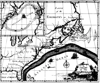
Figure 2.7 The 1786 version of Franklin-Folger map of the Gulf Stream.

beginning with the first scientific investigations of the 17th century. Initially progress was slow. First came very simple observations of far reaching impor-tance by scientists who probably did not consider themselves oceanographers, if the term even existed. Later came more detailed descriptions and oceanographic experiments by scientists who specialized in the study of the ocean.

1685 Edmond Halley, investigating the oceanic wind systems and currents, published “An Historical Account of the Trade Winds, and Monsoons, observable in the Seas between and near the Tropicks, with an attempt to assign the Physical cause of the said Winds”Philosophical Transactions.

1735 George Hadley published his theory for the trade winds based on con-servation of angular momentum in “Concerning the Cause of the General Trade-Winds”Philosophical Transactions, 39: 58-62.

1751 Henri Ellis made the first deep soundings of temperature in the tropics, finding cold water below a warm surface layer, indicating the water came from the polar regions.

1769 Benjamin Franklin, as postmaster, made the first map of the Gulf Stream using information from mail ships sailing between New England and Eng-land collected by his cousin Timothy Folger (figure 2.7).

(27)

1800 Count Rumford proposed a meridional circulation of the ocean with water sinking near the poles and rising near the Equator.

1847 Matthew Fontaine Maury published his first chart of winds and currents based on ships logs. Maury established the practice of international ex-change of environmental data, trading logbooks for maps and charts de-rived from the data.

1872–1876 Challenger Expedition marks the beginning of the systematic study of the biology, chemistry, and physics of the ocean of the world.

1885 Pillsbury made direct measurements of the Florida Current using current meters deployed from a ship moored in the stream.

1903 Founding of the Marine Biological Laboratory of the University of Cali-fornia. It later became the Scripps Institution of Oceanography.

1910–1913 Vilhelm Bjerknes published Dynamic Meteorology and Hydrogra-phy which laid the foundation of geophysical fluid dynamics. In it he developed the idea of fronts, the dynamic meter, geostrophic flow, air-sea interaction, and cyclones.

1930 Founding of the Woods Hole Oceanographic Institution.

1942 Publication ofThe ocean by Sverdrup, Johnson, and Fleming, a compre-hensive survey of oceanographic knowledge up to that time.

Post WW 2 The need to detect submarines led the navies of the world to greatly expand their studies of the sea. This led to the founding of oceanography departments at state universities, including Oregon State, Texas A&M University, University of Miami, and University of Rhode Is-land, and the founding of national ocean laboratories such as the various Institutes of Oceanographic Science.

1947–1950 Sverdrup, Stommel, and Munk publish their theories of the wind-driven circulation of the ocean. Together the three papers lay the foun-dation for our understanding of the ocean’s circulation.

1949 Start of California Cooperative Fisheries Investigation of the California Current. The most complete study ever undertaken of a coastal current. 1952 Cromwell and Montgomery rediscover the Equatorial Undercurrent in the

Pacific.

1955 Bruce Hamon and Neil Brown develop the CTD for measuring conduc-tivity and temperature as a function of depth in the ocean.

1958 Stommel publishes his theory for the deep circulation of the ocean.

1963 Sippican Corporation (Tim Francis, William Van Allen Clark, Graham Campbell, and Sam Francis) invents the Expendable BathyThermograph xbtnow perhaps the most widely used oceanographic instrument deployed from ships.

(28)

2.4. EVOLUTION OF SOME THEORETICAL IDEAS 15

1978 nasa launches the first oceanographic satellite, Seasat. The project de-veloped techniques used by generations of remotes sensing satellites.

1979–1981 Terry Joyce, Rob Pinkel, Lloyd Regier, F. Rowe and J. W. Young develop techniques leading to the acoustic-doppler current profiler for mea-suring ocean-surface currents from moving ships, an instrument widely used in oceanography.

1988 nasa Earth System Science Committee headed by Francis Bretherton outlines how all earth systems are interconnected, thus breaking down the barriers separating traditional sciences of astrophysics, ecology, geology, meteorology, and oceanography.

1991 Wally Broecker proposes that changes in the deep circulation of the ocean modulate the ice ages, and that the deep circulation in the Atlantic could collapse, plunging the northern hemisphere into a new ice age.

1992 Russ Davis and Doug Webb invent the autonomous, pop-up drifter that continuously measures currents at depths to 2 km.

1992 nasaandcnesdevelop and launch Topex/Poseidon, a satellite that maps ocean surface currents, waves, and tides every ten days, revolutionizing our understanding of ocean dynamics and tides.

1993 Topex/Poseidon science-team members publish first accurate global maps of the tides.

More information on the history of physical oceanography can be found in Ap-pendix A of W.S. von Arx (1962): An Introduction to Physical Oceanography.

Data collected from the centuries of oceanic expeditions have been used to describe the ocean. Most of the work went toward describing the steady state of the ocean, its currents from top to bottom, and its interaction with the atmosphere. The basic description was mostly complete by the early 1970s. Figure 2.8 shows an example from that time, the surface circulation of the ocean. More recent work has sought to document the variability of oceanic processes, to provide a description of the ocean suﬃcient to predict annual and interannual variability, and to understand the role of the ocean in global processes.

2.4 Evolution of some Theoretical Ideas

A theoretical understanding of oceanic processes is based on classical physics coupled with an evolving understanding of chaotic systems in mathematics and the application to the theory of turbulence. The dates given below are approx-imate.

19th Century Development of analytic hydrodynamics. Lamb’s Hydrodynam-ics is the pinnacle of this work. Bjerknes develops geostrophic method widely used in meteorology and oceanography.

(29)

Arctic Circle

East Australia

Alaska

California StreamGulf Labrador Florida Equator Brazil Peru or Humboldt Greenland Guinea Somali Benguala Agulhas Canaries Norway Oyeshio North Pacific Kuroshio North Equatorial Equatorial Countercurrent South Equatorial

West wind drift or Antarctic Circumpolar

West wind drift or Antarctic Circumpolar Falkland

S. Eq. C. Eq.C.C.

N. Eq. C.

S. Eq. C.

West Australia Murman Irminger North Atlantic drift

N. Eq. C. 60o 45o 30o 15o -15o -30o -45o -60o

0o C.C.

warm currents N. north S. south Eq. equatorial cool currents C. current C.C. counter current

Figure 2.8 The time-averaged, surface circulation of the ocean during northern hemisphere winter deduced from a century of oceanographic expeditions. After Tolmazin (1985: 16).

1940–1970 Refinement of theories for turbulence based on statistical correla-tions and the idea of isotropic homogeneous turbulence. Books by Batch-elor (1967), Hinze (1975), and others.

1970– Numerical investigations of turbulent geophysical fluid dynamics based on high-speed digital computers.

1985– Mechanics of chaotic processes. The application to hydrodynamics is just beginning. Most motion in the atmosphere and ocean may be inher-ently unpredictable.

2.5 The Role of Observations in Oceanography

The brief tour of theoretical ideas suggests that observations are essential for understanding the ocean. The theory describing a convecting, wind-forced, turbulent fluid in a rotating coordinate system has never been suﬃciently well known that important features of the oceanic circulation could be predicted before they were observed. In almost all cases, oceanographers resort to obser-vations to understand oceanic processes.

At first glance, we might think that the numerous expeditions mounted since 1873 would give a good description of the ocean. The results are indeed impressive. Hundreds of expeditions have extended into all ocean. Yet, much of the ocean is poorly explored.

(30)

2.5. THE ROLE OF OBSERVATIONS IN OCEANOGRAPHY 17

vastly under sampled. This is the sampling problem (See box on next page). Our samples of the ocean are insuﬃcient to describe the ocean well enough to predict its variability and its response to changing forcing. Lack of suﬃcient samples is the largest source of error in our understanding of the ocean.

The lack of observations has led to a very important and widespread con-ceptual error:

“The absence of evidence was taken as evidence of absence.” The great diﬃculty of observing the ocean meant that when a phenomenon was not observed, it was assumed it was not present. The more one is able to observe the ocean, the more the complexity and subtlety that appears— Wunsch (2002a).

As a result, our understanding of the ocean is often too simple to be correct.

Selecting Oceanic Data Sets Much of the existing oceanic data have been organized into large data sets. For example, satellite data are processed and distributed by groups working withnasa. Data from ships have been collected and organized by other groups. Oceanographers now rely more and more on such collections of data produced by others.

The use of data produced by others introduces problems: i) How accurate are the data in the set? ii) What are the limitations of the data set? And, iii) How does the set compare with other similar sets? Anyone who uses public or private data sets is wise to obtain answers to such questions.

If you plan to use data from others, here are some guidelines.

1. Use well documented data sets. Does the documentation completely de-scribe the sources of the original measurements, all steps used to process the data, and all criteria used to exclude data? Does the data set include version numbers to identify changes to the set?

2. Use validated data. Has accuracy of data been well documented? Was accuracy determined by comparing with diﬀerent measurements of the same variable? Was validation global or regional?

3. Use sets that have been used by others and referenced in scientific papers. Some data sets are widely used for good reason. Those who produced the sets used them in their own published work and others trust the data. 4. Conversely, don’t use a data set just because it is handy. Can you

doc-ument the source of the set? For example, many versions of the digital, 5-minute maps of the sea floor are widely available. Some date back to the first sets produced by the U.S. Defense Mapping Agency, others are from the etopo-5 set. Don’t rely on a colleague’s statement about the source. Find the documentation. If it is missing, find another data set.

Designing Oceanic Experiments Observations are exceedingly important

(31)

Sampling Error

Sampling error is the largest source of error in the geosciences. It is caused by a set of samples not representing the population of the variable being measured. A population is the set of all possible measurements, and a sam-ple is the samsam-pled subset of the population. We assume each measurement is perfectly accurate.

To determine if your measurement has a sampling error, you must first completely specify the problem you wish to study. This defines the popu-lation. Then, you must determine if the samples represent the popupopu-lation. Both steps are necessary.

Suppose your problem is to measure the annual-mean sea-surface tem-perature of the ocean to determine if global warming is occurring. For this problem, the population is the set of all possible measurements of surface temperature, in all regions in all months. If the sample mean is to equal the true mean, the samples must be uniformly distributed throughout the year and over all the area of the ocean, and suﬃciently dense to include all important variability in time and space. This is impossible. Ships avoid stormy regions such as high latitudes in winter, so ship samples tend not to represent the population of surface temperatures. Satellites may not sample uniformly throughout the daily cycle, and they may not observe tempera-ture at high latitudes in winter because of persistent clouds, although they tend to sample uniformly in space and throughout the year in most regions. If daily variability is small, the satellite samples will be more representative of the population than the ship samples.

From the above, it should be clear that oceanic samples rarely represent the population we wish to study. We always have sampling errors.

In defining sampling error, we must clearly distinguish between instru-ment errors and sampling errors. Instruinstru-ment errors are due to the inac-curacy of the instrument. Sampling errors are due to a failure to make a measurement. Consider the example above: the determination of mean sea-surface temperature. If the measurements are made by thermometers on ships, each measurement has a small error because thermometers are not perfect. This is an instrument error. If the ships avoids high latitudes in winter, the absence of measurements at high latitude in winter is a sampling error.

Meteorologists designing the Tropical Rainfall Mapping Mission have been investigating the sampling error in measurements of rain. Their results are general and may be applied to other variables. For a general description of the problem see North & Nakamoto (1989).

(32)

2.5. THE ROLE OF OBSERVATIONS IN OCEANOGRAPHY 19

The first and most important aspect of the design of any experiment is to determine why you wish to make a measurement before deciding how you will make the measurement or what you will measure.

1. What is the purpose of the observations? Do you wish to test hypotheses or describe processes?

2. What accuracy is required of the observation?

3. What resolution in time and space is required? What is the duration of measurements?

Consider, for example, how the purpose of the measurement changes how you might measure salinity or temperature as a function of depth:

1. If the purpose is to describe water masses in an ocean basin, then measure-ments with 20–50 m vertical spacing and 50–300 km horizontal spacing, repeated once per 20–50 years in deep water are required.

2. If the purpose is to describe vertical mixing in the open equatorial Pa-cific, then 0.5–1.0 mm vertical spacing and 50–1000 km spacing between locations repeated once per hour for many days may be required.

Accuracy, Precision, and Linearity While we are on the topic of experi-ments, now is a good time to introduce three concepts needed throughout the book when we discuss experiments: precision, accuracy, and linearity of a mea-surement.

Accuracy is the diﬀerence between the measured value and the true value.

Precision is the diﬀerence among repeated measurements.

The distinction between accuracy and precision is usually illustrated by the simple example of firing a rifle at a target. Accuracy is the average distance from the center of the target to the hits on the target. Precision is the average distance between the hits. Thus, ten rifle shots could be clustered within a circle 10 cm in diameter with the center of the cluster located 20 cm from the center of the target. The accuracy is then 20 cm, and the precision is roughly 5 cm.

Linearity requires that the output of an instrument be a linear function of the input. Nonlinear devices rectify variability to a constant value. So a non-linear response leads to wrong mean values. Non-non-linearity can be as important as accuracy. For example, let

Output=Input+ 0.1(Input)2

Input=asinωt

then

Output=asinωt+ 0.1 (asinωt)2

Output=Input+0.1

2 a

2₋0.1

2 a

2_{cos 2}_ω_t

(33)

twice the input frequency. In general, if input has frequencies ω1 andω2, then output of a non-linear instrument has frequencies ω1 ±ω2. Linearity of an

instrument is especially important when the instrument must measure the mean value of a turbulent variable. For example, we require linear current meters when measuring currents near the sea surface where wind and waves produce a large variability in the current.

Sensitivity to other variables of interest. Errors may be correlated with other variables of the problem. For example, measurements of conductivity are sensitive to temperature. So, errors in the measurement of temperature in salinometers leads to errors in the measured values of conductivity or salinity.

2.6 Important Concepts

From the above, I hope you have learned:

1. The ocean is not well known. What we know is based on data collected from only a little more than a century of oceanographic expeditions sup-plemented with satellite data collected since 1978.

2. The basic description of the ocean is suﬃcient for describing the time-averaged mean circulation of the ocean, and recent work is beginning to describe the variability.

3. Observations are essential for understanding the ocean. Few processes have been predicted from theory before they were observed.

4. Lack of observations has led to conceptual pictures of oceanic processes that are often too simplified and often misleading.

5. Oceanographers rely more and more on large data sets produced by others. The sets have errors and limitations which you must understand before using them.

6. The planning of experiments is at least as important as conducting the experiment.

7. Sampling errors arise when the observations, the samples, are not repre-sentative of the process being studied. Sampling errors are the largest source of error in oceanography.

(34)

Chapter 3 The Physical Setting

Earth is an oblate ellipsoid, an ellipse rotated about its minor axis, with an equatorial radius of Re = 6,378.1349 km (West, 1982) slightly greater than the polar radius of Rp = 6,356.7497 km. The small equatorial bulge is due to earth’s rotation.

Distances on earth are measured in many diﬀerent units, the most common are degrees of latitude or longitude, meters, miles, and nautical miles. Latitude

is the angle between the local vertical and the equatorial plane. A meridian is the intersection at earth’s surface of a plane perpendicular to the equatorial plane and passing through earth’s axis of rotation. Longitude is the angle between the standard meridian and any other meridian, where the standard meridian is the one that passes through a point at the Royal Observatory at Greenwich, England. Thus longitude is measured east or west of Greenwich.

A degree of latitude is not the same length as a degree of longitude except at the equator. Latitude is measured along great circles with radiusR, where R is the mean radius of earth. Longitude is measured along circles with radius Rcosϕ, where ϕ is latitude. Thus 1◦

latitude = 111 km, and 1◦

longitude = 111 cosϕkm.

Because distance in degrees of longitude is not constant, oceanographers measure distance on maps using degrees of latitude.

Nautical miles and meters are connected historically to the size of earth. Gabriel Mouton proposed in 1670 a decimal system of measurement based on the length of an arc that is one minute of a great circle of earth. This eventually became the nautical mile. Mouton’s decimal system eventually became the metric system based on a diﬀerent unit of length, the meter, which was originally intended to be one ten-millionth the distance from the Equator to the pole along the Paris meridian. Although the tie between nautical miles, meters, and earth’s radius was soon abandoned because it was not practical, the approximations are very good. For example, earth’s polar circumference is approximately 40,008 km. Therefore one ten-millionth of a quadrant is 1.0002 m. Similarly, a nautical mile should be 1.8522 km, which is very close to the oﬃcial definition of the

international nautical mile: 1 nm≡1.8520 km.

(35)

22 CHAPTER 3. THE PHYSICAL SETTING

-80o _-40o ₀o ₄₀o

-90o -60o -300 00

30o 60o

90o

-4000 -3000 -1000 -200 0

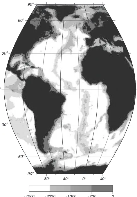
Figure 3.1 The Atlantic Ocean viewed with an Eckert VI equal-area projection. Depths, in meters, are from theetopo30′ _{data set. The 200 m contour outlines continental shelves.}

3.1 Ocean and Seas

There is only one ocean. It is divided into three named parts by international agreement: the Atlantic, Pacific, and Indian ocean (International Hydrographic Bureau, 1953). Seas, which are part of the ocean, are defined in several ways. I consider two.

The Atlantic Ocean extends northward from Antarctica and includes all of the Arctic Sea, the European Mediterranean, and the American Mediter-ranean more commonly known as the Caribbean sea (figure 3.1). The boundary between the Atlantic and Indian Ocean is the meridian of Cape Agulhas (20◦

E). The boundary between the Atlantic and Pacific is the line forming the short-est distance from Cape Horn to the South Shetland Islands. In the north, the Arctic Sea is part of the Atlantic Ocean, and the Bering Strait is the boundary between the Atlantic and Pacific.

(36)

3.2. DIMENSIONS OF THE OCEAN 23

1 2 0o ₁₆₀o _-160o _-120o _{- 8 0}o

-90o

-60o

-30o

0o

30o

60o

90o

-4000 -3000 -1000 -200 0

Figure 3.2 The Pacific Ocean viewed with an Eckert VI equal-area projection. Depths, in meters, are from theetopo30′ _{data set. The 200 m contour outlines continental shelves.}

line from the Malay Peninsula through Sumatra, Java, Timor, Australia at Cape Londonderry, and Tasmania. From Tasmania to Antarctica it is the meridian of South East Cape on Tasmania 147◦

E.

The Indian Ocean extends from Antarctica to the continent of Asia in-cluding the Red Sea and Persian Gulf (figure 3.3). Some authors use the name Southern Ocean to describe the ocean surrounding Antarctica.

Mediterranean Seas are mostly surrounded by land. By this definition, the Arctic and Caribbean Seas are both Mediterranean Seas, the Arctic Mediter-ranean and the Caribbean MediterMediter-ranean.

Marginal Seasare defined by only an indentation in the coast. The Arabian Sea and South China Sea are marginal seas.

3.2 Dimensions of the ocean

(37)

40o ₈₀o ₁₂₀o

-90o -60o -30o 0o

30o

-4000 -3000 -1000 -200 0

Figure 3.3 The Indian Ocean viewed with an Eckert VI equal-area projection. Depths, in meters, are from theetopo30′ _{data set. The 200 m contour outlines continental shelves.}

Oceanic dimensions range from around 1500 km for the minimum width of the Atlantic to more than 13,000 km for the north-south extent of the Atlantic and the width of the Pacific. Typical depths are only 3–4 km. So horizontal dimensions of ocean basins are 1,000 times greater than the vertical dimension. A scale model of the Pacific, the size of an 8.5×11 in sheet of paper, would have dimensions similar to the paper: a width of 10,000 km scales to 10 in, and a depth of 3 km scales to 0.003 in, the typical thickness of a piece of paper.

Because the ocean is so thin, cross-sectional plots of ocean basins must have a greatly exaggerated vertical scale to be useful. Typical plots have a vertical scale that is 200 times the horizontal scale (figure 3.4). This exaggeration distorts our view of the ocean. The edges of the ocean basins, the continental slopes, are not steep cliﬀs as shown in the figure at 41◦

W and 12◦

E. Rather, they are gentle slopes dropping down 1 meter for every 20 meters in the horizontal.

The small ratio of depth to width of the ocean basins is very important for understanding ocean currents. Vertical velocities must be much smaller

Table 3.1 Surface Area of the ocean †

Pacific Ocean 181.34×106

km2

Atlantic Ocean 106.57×106 _km2

Indian Ocean 74.12×106

(38)

3.3. SEA-FLOOR FEATURES 25

Depth (km)

-45o _-30o _-15o ₀o ₁₅o

-6 -4 -2 0

Longitude

6 km 6 km

-45o _-30o _-15o ₀o ₁₅o

Figure 3.4 Cross-section of the south Atlantic along 25◦_{S showing the continental shelf}

oﬀshore of South America, a seamount near 35◦_{W, the mid-Atlantic Ridge near 14}◦_{W, the}

Walvis Ridge near 6◦_{E, and the narrow continental shelf oﬀ} _{South Africa.} _Upper _Vertical

exaggeration of 180:1. LowerVertical exaggeration of 30:1. If shown with true aspect ratio, the plot would be the thickness of the line at the sea surface in the lower plot.

than horizontal velocities. Even over distances of a few hundred kilometers, the vertical velocity must be less than 1% of the horizontal velocity. I will use this information later to simplify the equations of motion.

The relatively small vertical velocities have great influence on turbulence. Three dimensional turbulence is fundamentally diﬀerent than two-dimensional turbulence. In two dimensions, vortex lines must always be vertical, and there can be little vortex stretching. In three dimensions, vortex stretching plays a fundamental role in turbulence.

3.3 Sea-Floor Features

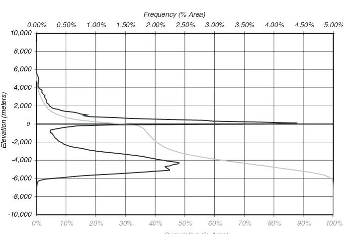
Earth’s rocky surface is divided into two types: oceanic, with a thin dense crust about 10 km thick, and continental, with a thick light crust about 40 km thick. The deep, lighter continental crust floats higher on the denser mantle than does the oceanic crust, and the mean height of the crust relative to sea level has two distinct values: continents have a mean elevation of 1100 m, the ocean has a mean depth of -3400 m (figure 3.5).

(39)

0

-10,000 -8,000 -6,000 -4,000 -2,000 2,000 4,000 6,000 8,000 10,000

Ele

va

tio

n

(

meters)

0% 10% 20% 30% 40% 50% 60% 70% 80% 90% 100%

Cumulative (% Area)

0.00% 0.50% 1.00% 1.50% 2.00% 2.50% 3.00% 3.50% 4.00% 4.50% 5.00% Frequency (% Area)

Figure 3.5 Histogram of height of land and depth of the sea as percentage of area of earth in 100 m intervals, showing the clear distinction between continents and sea floor. The cumulative frequency curve is the integral of the histogram. The curves are calculated from theetopo2 data set by George Sharman of thenoaaNational Geophysical Data Center.

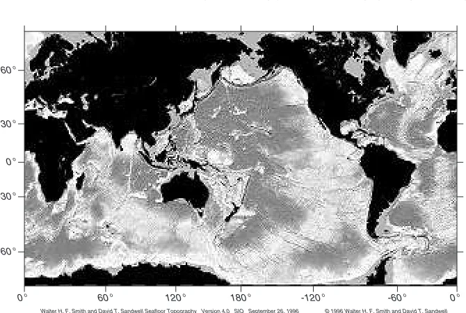
The crust is broken into large plates that move relative to each other. New crust is created at the mid-ocean ridges, and old crust is lost at trenches. The relative motion of crust, due to plate tectonics, produces the distinctive features of the sea floor sketched in figure 3.6, including mid-ocean ridges, trenches,

is-Shore

High Water Low Water

Sea Level

OCEAN SHELF

(Gravel, Sand Av slope 1 in 500)

SLOPE

(Mud av slope 1 in 20)

CONTINENT

RISE

BASIN

MID-OCEAN RIDGE

DEEP SEA (Clay & Oozes)

Mineral Organic SEAMOUNT

TRENCH ISLAND ARC

(40)

3.3. SEA-FLOOR FEATURES 27

land arcs, and basins. The names of the sub-sea features have been defined by the International Hydrographic Organization (1953), and the following defini-tions are taken from Sverdrup, Johnson, and Fleming (1942), Shepard (1963), and Dietrich et al. (1980).

Basins are deep depressions of the sea floor of more or less circular or oval form.

Canyonsare relatively narrow, deep furrows with steep slopes, cutting across the continental shelf and slope, with bottoms sloping continuously downward.

Continental shelves are zones adjacent to a continent (or around an island) and extending from the low-water line to the depth, usually about 120 m, where there is a marked or rather steep descent toward great depths. (figure 3.7)

Continental slopesare the declivities seaward from the shelf edge into greater depth.

Plains are very flat surfaces found in many deep ocean basins.

Ridges are long, narrow elevations of the sea floor with steep sides and rough topography.

(41)

21.4o

21.3o

21.2o

21.1o

21.0o

20.9o

20.8o

163.0o

163.1o

163.2o

163.3o

163.4o

163.5o

163.6o 40

20

14

40

40 20

40

48

30

Figure 3.8 An example of a seamount, the Wilde Guyot. A guyot is a seamount with a flat top created by wave action when the seamount extended above sea level. As the seamount is carried by plate motion, it gradually sinks deeper below sea level. The depth was contoured from echo sounder data collected along the ship track (thin straight lines) supplemented with side-scan sonar data. Depths are in units of 100 m. From William Sager, Texas A&M University.

Seamountsare isolated or comparatively isolated elevations rising 1000 m or more from the sea floor and with small summit area (figure 3.8).

Sills are the low parts of the ridges separating ocean basins from one another or from the adjacent sea floor.

Trenches are long, narrow, and deep depressions of the sea floor, with rela-tively steep sides (figure 3.9).