Design and Implementation of a Nonlinear
H
∞
tracking Controller for high Elastic
Joint Robot with Compensated Friction
M.A.Akbari† G.Alizadeh† S.Khanmohammadi† I.Hassanzadeh† M.Mirzaei†† M.A.Badamchizadeh††Faculty of Electrical and Computer Engineering University of Tabriz, Tabriz, IRAN
††Faculty of Mechanical Engineering, University of Sahand, Tabriz, IRAN †{makbari,alizadeh,khan,izadeh,mbadamchi}@tabrizu.ac.ir
††[email protected] Abstract:
This paper proposes a nonlinear H∞tracking controller to control a laboratory rotary single link elastic joint robot which has tolerances on mechanical parameters. The elastic property of joint is performed by means of a solenoid spring which is connected between actuator shaft and joint of link as bilateral structure. The new smooth model is used for modeling of frictions which is compatible with numerical algorithms. It is shown that the effect of coulomb friction and gearbox backlashes are decreased by using a pulsation signal as an extra voltage that is added to the control voltage of actuator. Also in this paper a smooth model is used for modeling saturation on actuator. The control law is calculated as a function of end payload by using Taylor expansion algorithm on final smooth model. Experimental results express that the proposed controller has ability to stable and control single link elastic joint robot with a good performance.
Keywords: nonlinear H;high elastic joint robot; saturation; friction.
1. Introduction
Flexible robot systems are usually used in the aerospace industry, chemical processing, integrated circuits manufactured and nuclear energy plants to execute commands with high sensitivity and accuracy [1] . Hence a high-accurate controlling requires to new structures [2] . Traditional controllers with linear structure are still used in robotics with low performance and weak stability. Like to majority electro-mechanical systems, there are uncertainty in model of flexible robots because of tolerance of physical parameters. For years, efforts have been made to design convenient controllers to solve this problem such as robust, adaptive and intelligent controllers [3] . Robust controllers are considered as one of the most reliable controllers in this area. Linear H∞ (L-H∞) as a useful robust controller is used to control linear systems with bounded disturbance and uncertainty. In most cases the L-H∞ controller is also used to control nonlinear systems with weak nonlinearity. But it is unfeasible to design a single controller by L-H∞ for flexible robots because of their high nonlinearity. Such systems may be unstable in out of working space. High overshoot and undershoot are some of disadvantages of such controllers. Nonlinear H∞ (NL-H∞) was proposed by Van der shaft and a number of other scientists in 1990’s for nonlinear systems [4] , afterward this method was improved by others among Isidori and colleagues [5] . Internal stability and L2-gain performance on closed loop system are two purposes in NL-H∞ theory [4] .In order to design a NL-H∞ controller, it is required to solve a nonlinear partial differential equation which is called Hamilto n-Jacobi-Equation (HJE) [4] . In general there is no analytical solution for HJE. The regular method based on Taylor series was proposed to solve HJE by Huang and Liu [6] . Lu and Doyle proposed a new solution based on nonlinear in-equation matrices instead of HJE [7] . For the first time, Fu and Nguang studied on uncertainty problem in nonlinear systems [8] . As robust control view, they found out that Flexible Joint Robots (FJR) are a good case to control by NL-H∞ method [9] . In practice, FJRs describing model have uncertainties because tolerances of length and mass of links, gearboxes parameters and springs stiffness coefficient. Moreover mechanical and electrical parameters of electromagnetic actuators insert extra uncertainty to final model.
systems with backlashes property may cause instability in closed loop system. Moreover, it is usual that motor out-torque is transferred by special gearbox, which is called harmonic-drive, from actuator to joint. Harmonic-drive has some flexibility similar to spring. Saturation in actuator is another important problem especially in high accelerations. Often this problem occurs because lightweight FJR is constructed by use of low power actuator.
2. Modeling
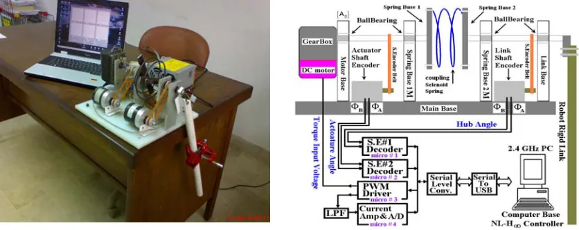
In this paper, the process of designing of a robust controller for a single link FJR is proposed. The scheme of the single link FJR is shown in figure 1. Which includes rigid arm, flexible joint and actuator. Usually actuator is a combination of gearbox and electromagnetic motor as a compact unit fixed on the work-table by a rigid base. Several fixed ball-brings on parallel bases are used to fixing shafts and reducing effect of friction. Gearbox generated torque is transferred by fixed shafts from gearbox-out to input of spring and from output of spring to joint of link. Solenoid type spring is selected for coupling [11] . In subsection 2.4 it will be shown this spring is employed in torsion form and also has weak nonlinearity.
Fig.1. Scheme of a single link FJR
2.1. FJRs Base model
Dynamic models for link and actuator sections can be created by two Lagrange differential equations as follows [13]:
i i
i
i i
i i i i i i i i
L
L
d
u
i 1 ; link of system
dt
i 2 ; actuator of system
L
,
,
p
(1)Where i, piand ui are as follows. For link:
1 1 L 1 P 1
2 2
1 1 1 L 1 P 1
1 C FL E1
1
p
m .g. .cos( ) m .g. .cos( )
2
1
1
,
I
m
2
2
u
u
u
u
(2)For actuator:
2 2
2
2 2 2 2
2 in C Fa E2
p
0
1
,
J.
2
u
u
u
u
u
(3)Where uE1, uE2 and uFa , uFL are axles position shaft-encoders torques and friction torques of link and actuator.
, mP, IL and J are mass of link, payload, inertia moment of arm and actuator respectively. Also ℓ, g , 1 and 2
are the length of arm , the gravity acceleration constant, the rotation angle of link and actuator-shaft to system base respectively. By replacing L1and L2 in the Lagrange equations in Eq.(1) FJR dynamics is described by:
2
L P 1 L P 1 C FL E1
2 2 in C Fa E2
1
I
m
m
m g. .sin( ) u
u
u
2
J.
B.
u
u
u
u
(4)
2.2. Friction smooth modeling
As it was mentioned uFa , uFL are friction torques in the link and actuator which are generated by viscous and
Coulomb frictions. Dynamic of friction torques can be written as [13] :
FL VL 1 CL
Fa Va 2 Ca
u
F .
u
u
F .
u
(5)Generally FVL ,FVa are constants which are related to type of surfaces and quality of lubrication. Usually, using
lubrication and ball-brings can decrease Coulomb friction on the joint and arm sections. But lubrication cannot be used in brushing of DC motor, so Coulomb friction has high value in gearbox and motor section. In this paper, uCa is selected as follows [13] :
f 2 2
Ca in in f
2
f in
C .sgn( )
;
0
1
u
u
; u
W.S
0
W
S .sgn(u ) ; otherwise
(6)Where Cf , Sf , uin and W are coefficient of kinetic and static frictions, applied torque and proportional weight
respectively. It is also proved that Coulomb friction is generated by kinetic and static frictions and generally Cf
is less than Sf. Often, designing a nonlinear controller for nonlinear systems will be conducted to use of
numerical methods, so dynamic equations should have Taylor expansion. There is no Taylor series for equations similar to Eq.(6), because it has some non derivativeable points on defined domain. This problem can be solved by using the following approximate equation [13] instead of Eq.(6). This equation is derivativeable in all defined domain.
2
Ca f 2 2 2
2
A.
u
C tanh(C. )
;
1 B.
(7)Also Sf in Eq.(6), which has positive value, is functions of A, B and Cf as follows: 2
f f 2 2
2
A.
S
Max C tanh(C. )
1 B.
(8)Where, C is a positive number which represents the slope of uCa in low speeds. Lubrication on ball-brings and
gearbox is usually used in order to decrease Cf and Sf. But lubrication is not possible between collector and
coals in DC and universal motors, because it may cause electrical conductivity problem. Based on Eq.(6), Coulomb friction torque have high value at low speeds, so if rotor rotates without stopping, then starting torque is eliminated and Coulomb friction is decreased which is shown experimentally in section 4.
2.3. Saturated motor modeling
m m b m m b m
out motor
a (Max)
K
V
K
V
K
u
.tanh
Ls R
(Ls R)i
(9)
Where ia , Km and ia(Max) are armature current, positive value as armature current to out-torque conversion
constant and maximum allowable current in armature respectively. If the armature current is equal or greater than the maximum allowable current, saturation would happen in rotor and stator cores. In this paper saturation is modeled by smooth function tanh(.) as an approximation of saturation dynamics. uout-motor is applied to input of
coupling spring as uin. Also R, L, Vm, m and Kb are armature resistance, armature inductance, input voltage,
motor speed at gearbox out, and speed to back e.m.f voltage conversion constant respectively. Figure 2 shows a model of DC motor that is used as robot actuator. In this model motor input voltage is a mixture of nonlinear controller output and symmetric pulse vibration voltages.
Fig.2. Model of DC motor and input mixed voltage Fig.3. Tensional and Spastic modes
2.4. Coupling model
In FJRs flexible gearbox out-torques is applied to robot joint as actuator. But in this paper, flexible gearbox was replaced by a set of rigid gearbox and tortuous solenoid spring for having high flexibility. In this working mode, spring coefficient is very low. Other problem, which complicates designing process, is nonlinearity of spring. As it is shown in figure 3, effective diameter of spring can be changed in Tensional and Spastic modes, because distance of spring bases is always fixed.
Increasing and decreasing in spring diameter on Tensional and Spastic modes can cause higher nonlinearities in FJRs specifications and also model may become asymmetric according to the following equations [15] :
3 5
c 1 3 5
c 3 5
c 1 3 5
2 1 1 2
i i i i
u
a
a
a
;
0
u
u
a
a
a
;
0
|
and
a
a
0 or a
a
0 ; i 1,3,5
(10)All
a
i+ anda
i- are Tensional and Spastic modes' polynomial coefficients. In Eq.(10) it is assumed that coefficients of even powers of uc and c
u polynomials are all zero, because of symmetric structure to origin.
Generally Eq. (10) is not derivable on the origin; therefore it will not have Taylor expansion. In order to eliminate conflicting, the following equation can be used instead of Eq.(10) in defined domain as a continues and derivable approximation.
3 5
1 3 5
c
a
ˆ
a
ˆ
a
ˆ
u
(11)Where ˆa are new polynomial coefficients with uncertainty that are bounded between lower and upper size i
ofˆa . Therefore i ˆa can be defined based on i
a
i+ and a
i i ai
i i
i i i i i
i i
ai
i i
ˆa
a (1 w )
a
a
a
a & a
or a & a
2
a
a
w
a
a
(12)Where wai represents maximum deviation
a
i+ and ai- froma
i. Figure 4 shows how to connect spring to bases. In this paper a new method is proposed for symmetrical transferring of torque from actuator to spring where 50% of coupled torque is applied to the spring at A by OA link and the rest is applied to A' by OA' link and the fixed arc of spring (AA'). Spring properties, may changed if connection points (A, A') are fixed by high temperature methods such as soldering. Therefore to avoid this problem spring and bases were fastened by screws and spanners in laboratory experiments. Also applied force on connection points (A, A') is equal to u OA1 whichcan be reduced by incrementing the bases length (OA, OA'). This structure has some advantages such as symmetrical transmission for torque by two sides of spring bases, decrease in applied forces on connection points and decrease in friction forces over boll brings.
Fig.4. Symmetric connection for spring and gearbox shaft
3. Uncertainty and
NL H
controllerIn this section the new model of FJR is presented, which has uncertainty as tolerance of parameters and disturbance inputs. The FJR model must be converted to new structure, because of compatibility with NLH
theory. It is also assumed that states of system are full available and system equations in state space are described as follows [6] :
1 2
x f (x) g (x)w g (x)u
z h(x) l(x)u
(13) Where, xRnis the state vector, wRm1is the disturbance input vector, uRm2is the control input vector
and zRpis the penalty variable vector. Also, it is assumed that functions f(x),g1(x),g2(x),h(x),l(x) are defined and are smooth in the neighborhood of X on Rn.
3.1.
NL
H
and uncertainty modelingTo design a controller based on NLH theory it is need that system dynamics must be expressed state space
form. If state vector of system is defined as:
1 2 3 4 5 6 1 1 2 2 a
x x
[
x
x
x
x ] [
i
e.dt]
(14)1 2
2 2 1 2 3
3 4
4 4 1 3 4 5
5 5 4 5 25 m
6 d 1
x
x
ˆ
x
f (x , x , x , w)
x
x
ˆ
x
f (x , x , x , x , w)
ˆ
x
f (x , x , w) g (x).V
x
x
x
(15)These equations are written by using Eq. (4),(5),(9),(11). Where ˆw is the input disturbance vector. Also the models of shaft encoders were eliminated for simplicity, because of their low effects. Equation for x6 is added
to FJR describing equations to decrease the tracking error. Where xd and x6 are the input command as desired
position and integral of tracking error. In this paper, tolerances of mechanical parameters such as mass and length of link are also considered, because these parameters can be changed easily. It is assumed that measuring of fixed mechanical and electrical parameters in compact motor and gearbox have been done with enough precision. Tolerance of parameters can be defined as follows:
L 1 1 1
P 2 2 2
1 3 3
m
m (1
w )
m
m (1
w )
(1
w )
(16)
Where, 1,2and 3 are positive numbers as maximum deviations of mL, mP and respectively. Also w1, 2
w and w3 are external input signals, which are limited by |wi|<1. Therefore ˆw is defined as follows:
T1 2 3 a1 a3 a5 d
ˆw
w , w , w , w , w , w , x
(17) In order to have compatibility between FJR model and NLH equations structure, it is necessary that5 4 2
f ,f ,f will be expressed as follows [6] :
i
ˆ
i 1iˆ
f (x, w) f (x) g (x).w ; i 2, 4,5, 6
(18)Where f (x)i and g (x)1i are:
ˆ
i i w 0
1i 1i1 1i2 1i3 1i4 1i5 1i6
i
ˆ
1ij w 0
j
ˆ
f (x) f (x, w) |
g (x)
g
g
g
g
g
g
i 2, 4,5, 6
ˆ
f (x, w)
g
|
;
j 1,...,6
w
(19)Also in this paper, h(x) was selected as follow:
Tx1 1 x 2 2 6 6
h(x)
Q x
Q x
0 0 0 Q x
(20)Where Q6 can be used as tracking accuracy setting, Qx1 and Qx 2 can be adjusted for having the least overshoot
on the system response. For simplicity in controller designing the follows assumption is made:
T
2
l (x)l(x) R
(21)Where R2 is a nonzero constant. Therefore NLHcontrol law can be calculated as [6] :
1 T T
m 2 2 x
V
R g (x)V
(22)Where Vx is the gradient ofV(x) which is a positive define function of stat vector so that must satisfy locally the following differential equation in the neighborhood of origin inRn.
T
T 1 1 1 T
x x 2 2 2 2 x
g g
1
1
V f (x)
h h
V (
g R g )V
0
2
2
Therefore attenuation of disturbance signals is done by scale. Because of non-linear nature of system, there is a low possibility to find a closed analytical solution for Eq.(23). In most cases, the numerical solution is used instead of the analytical solution.
3.2.
NL
H
controller by Taylor expansion algorithmAlso as it was mentioned, in most cases it is needed for Taylor expansion for calculating NLHbased control
law for nonlinear systems. According to the proposed algorithm in [16] , it is assumed V(x)in Eq.(23) has the following structure:
T [k]
k k 3
1
V(x)
x Px
P x
2
(24)Therefore control signal (motor applied voltage) can be generated by:
[k]
m 1 k
k 3
V
Q .x
Q .x
(25)Where Q1 and Qk can be calculated by using P , Pk and the proposed equations in [16] . Pn n is a
symmetric positive define matrix that is calculated by the following Riccati's equation:
T T 1 T T
2 2 2 2 1 1
1
A P PA C C P B R B
B B P 0
(26)1 2
A, C, B , B are matrixes that can be created by linearization of system on equilibrium point as follows:
[2 ] [2 ]
[1 ] [1 ]
1 1 1 2 2 2
f (x) Ax f
(x) , h(x) Cx h
(x)
g (x) B
g
(x) , g (x) B
g
(x)
(27)[2 ] [2 ]
f (x) , h (x) consist of the second and higher order terms of f (x), h(x) and [1 ] [1 ]
1 2
g (x) , g (x) consist of the first and higher order terms of g (x),g (x) . Also, in this algorithm 1 2
[k]
x is generated by using Kroniker product of nonlinear system states. Deviation of most parameters in the system is so small and bounded that they can be considered the same as disturbance inputs. Unlike to them, the value of mP can be changed in a
wide range. Hence, it is impossible that a unique controller will be found based on NLH theory for wide
varying of payload value. An ideal and general purpose controller must be function of all effective system parameters as:
m L P m b
V
f x, m , m , I, k, J, B, , R, L, K , K , ...
(28)But in most cases, it is impossible. So instead of analytic solutions, using of numerical solutions is often proposed. But approximate solutions can formulate the control law as a function of system states. Therefore
k
P , P are constant matrix and vector. In this paper, the following equations are used instead of Eq.(25) in order to solve the wide changing problem in payload:
m P
V
f x, m
(29)Where Pand Pk are positive define matrix and a vector that are functions of states and mP . Therefore, V(x)
will have the following structure:
T [k]
P k P
k 3
1
V(x)
x P(m )x
P (m )x
2
(30)and signal control is as:
[k]
m 1 p k p
k 3
V
Q [m ].x
Q [m ].x
(31) Improved performance controller for wide changing of payload. No need for frequently calculations.
Decreasing in controller time delay by eliminating some of the low effect sentences. 4. Experimental Results
In order to analyze the proposed controller performance, a single flexible joint robot test-bed was prepared in University of Tabriz. This FJR has two main sections, electro-mechanic and control sections. Electro-mechanic section is split to compact gear-boxed DC motor as actuator, solenoid spring as torque transformer and plastic rigid link as arm. Also, in order to avoid undesired movements, main shaft from gearbox output to joint of arm is fastened by fixed parallel bases on main foundation. Controller section has four high speed micro-controllers. Gearbox-shaft and link positions are measured by high precision shaft encoders as measured output signals. Shaft encoders signal wires are connected to two separable and independent micro-controllers as inputs. These outputs are wired to the interrupt inputs of micro-controllers. Outset, the pulses of shaft-encoders are decoded and then rotational angles are separately calculated by a special algorithm in micro-controllers. In the next phase, decoded information is sent to main computer by RS232 protocol as serial communication and serial to USB converter. The main controller is a software controller programmed in Visual Basic. The controller on main computer gets gearbox-shaft and link positions by serial line and control law coefficients of a file that was already created by the other program in MATLAB.
Fig.5. Photo and scheme of single link FJR and controller test-bed
Special numerical code as DC motor voltage is created by use of control law and positions information in controller. Then this code is sent to the fourth microcontroller by serial line. In order to create apposite commands for generating PWM form DC voltage as motor power supply. DC voltage is generated by four IGBTs as a controllable bridge and PWM method. According to the controller commands produced voltage can be altered in range 24 to 24V V.
4.1. Laboratory FJR parameters
Table 1 shows values of compact gear-boxed DC motor set electrical and mechanical parameters. Table 1. Compact DC motor and gearbox set properties
Parameters Nominal values Tolerance
Coil resistance r=9 ohm 4%
Coil inductance l=0.1 H 5%
Torque const. km=3.3 3%
Back emf const. kb=5.62 3%
Gearbox ratio N=100 : 1 -
Motor inertia J=2.15 3%
Operating Max. Voltage V=36 - Max. armature current A
a
Also, Table 2 shows values of link and spring mechanical parameters. Table 2. Link and spring properties
Parameters Nominal values Tolerance
Joint stiffness a13.35 1.5% 3
a 0.16 97%
Link Length L=0.53 6%
Link mass M=0.12 9%
Gravity coefficient g=9.8 1%
Inertia I=0.083 4%
Coulomb and viscose friction coefficients are presented for link and compact gear-boxed DC motor in Table 3. This table also shows coefficients at two states: without vibration and with vibration signal. Of course vibration signal had proper quantities during experimentally tests.
Table 3. Values of friction coefficients
Parameters No- vibration with- vibration
Link Coulomb const. Fc-link=.05 -
Link Viscose const. Fv-link=0.1 -
Motor Viscose const. Fv-motor=1.43 -
Motor coulomb const. Cf 0 .8 3 , c1 , B9 , A 3 .6 Cf 0 .3 , c1 , B3 .1 , A 1 .5
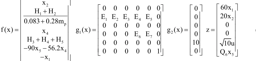
4.2. System dynamics as a function of payload
f (x) , g (x)1 , g (x)2 and z(x, u) for test-bed dynamics are created Based on NL-H∞ theory and proposed
models as a function of m and state vector by use of Tables 1,2,3. These functions are as follows: p 2
1
1 2
2
1 2 3 4 5
p
1 2
4
6 7
3 4 5
5 4
6 5 1
x
60x
0 0 0 0 0 0
0
H
H
20x
E E E E E 0
0
0.083 0.28m
0 0 0 0 0 0
0
0
f (x)
x
g (x)
0 0 0 E E 0
g (x)
0
z
0
H
H
H
0 0 0 0 0 0
10
10u
90x
56.2x
0 0 0 0 0 1
0
Q x
x
(32)
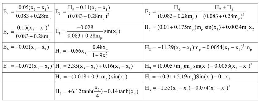
More details of mentioned functions were written in appendix A. 4.3. Nonlinear controller as a function of payload
In order to calculate Q1 and Q3 as a function of mp, Taylor expansion algorithm is used several times for kg
p
m [0.1,0.2,...,0.9] . Therefore test-bed control law will have a compatible structure with Eq.(31) up to k=3. So,Q [m ]1 p and Q [m ]3 p can be written as a function of payload value as following equations:
T
T1 p 1 p 3 p 3 p
Q [m ]
S .M
, Q [m ]
S .M
(33)Therefore applied voltage to motor will have following law:
T
T [k]m 1 p 3 p
V
S .M
.x
S .M
.x
(34)Where S1 and S3 are 6 6 and 56 4 matrix and Mp is a vector of m as follow: p T
3 2
p p p p
M
m
m
m
1
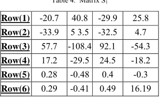
(35)S1 and S3 are calculated by interpolation on simulation results. Table 4 shows the values of S1 . In order to
Table 4. Matrix S1
Row(1) -20.7 40.8 -29.9 25.8 Row(2) -33.9 5 3.5 -32.5 4.7 Row(3) 57.7 -108.4 92.1 -54.3 Row(4) 17.2 -29.5 24.5 -18.2 Row(5) 0.28 -0.48 0.4 -0.3 Row(6) 0.29 -0.41 0.49 16.19
Some of the coefficients are independent of mp such as x6, because value of that is independent of p
m .Moreover some of the other coefficients have linear or quadratic relation with mp.
4.4. Compensated model for frictions
The results of tests show that the friction model can be compensated by applying a pulsation form signal (vibration signal) with special frequency and amplitude. Table 5 shows values of S , Cf f by some vibration
signals. These tables were gathered by various experimentally tests on test-bed L-FJR. Table 5. SfandCffor some vibration signals
( . ) . ( . ) .
f f
S N Vib 0 98 C N Vib 0 82
6vp p 4vp p 2vp p
f
S Cf Sf Cf Sf Cf
5Hz 0.37 0.27 0.27 0.2 0.68 0.55 10Hz 0.4 0.24 0.29 0.23 0.52 0.46 15Hz 0.39 015 0.35 0.3 0.63 0.52 4.5. Low effected backlash by vibration signal
In order to show advantages of proposed controller with vibration signal, a number of tests were done on L-FJR for various input commands.
Fig.6. Link position and tracking error for step command 90' with vibration signal
Figure 6 shows that response to step command 90' with vibration signal is more accurate than without it and also shows that link angle was sat to input command at t=8s by vibration signal, but it has ringing form on response
for without vibration signal even after t=16s. Also tracking error of two conditions is shown in figure 6.
4.6. Wide changing in payload
In order to show advantages of proposed controller law to traditional. The other tests were done on L-FJR by use of three different payloads. Figure 7 shows the test results of controller k(x, m ) and k(x) in the same p
conditions. Similar to subsection 4.4, optimal vibration signal has been applied in these tests.
It can be concluded from figure 7 that new controller has more compatibility with mp. Also, in addition to solve
Fig.7. Effect of mp changing with k(x, m )p and k(x)
Uncertainties and disturbance
Robustness of the proposed controller is verified by several experimentally tests. The tests have been conducted by changing the link length. Figure 8 shows the step response of link position in controlled system by proposed control law for link uncertainties. Also it shows the response of link position to step command 60', where external disturbances are applied as an impact forces to link. The results of tests show that the proposed controller can guarantee the system stability against parameter tolerances and external disturbances.
Fig.8. Link position for step command 60' with external disturbance and link uncertainty
Fig.9. Applied voltage to DC motor and control energy for step command 120'
Motor applied voltage and control energy are shown in figure 9. They are measured in two modes: with vibration signal and without vibration signal. Figure 9 shows that if motor control voltage is mixed with vibration signal, motor applied voltage will have smooth function with low variations after t=6s and also control
and desirable, because generated control signals by NLH controller have been practically applied to motor during tests without any problem.
5. Conclusion
This paper proposed a new structure to construct a laboratory single link FJR. L-FJR was controlled by using a new robust controller based onNLH theory which was a function of end payload. The backlashes and high starting torque problems in gear-boxed motor were decreased by use of vibration signal. Also the effect of Coulomb friction was decreased by using vibration signal. Moreover in this paper, actuator saturation and Coulomb friction were modeled by derivable and smooth equations. Experimental results of proposed controller on L-FJR shown that proposed controller enhanced performance of traditional NLHbased controller. The proposed approach can be expanded as a powerful technique to the more challenging cases of systems with unstable dynamics such as multilink flexible joint and link robots.
References
[1] Siciliano, B., “Control in Robotics: Open Problems and Future directions,” Proc. IEEE Int. Conf. on Cont. Applications, 1998 [2] Spong, M.W., K. Khorasani, and P.V. Kokotovic, “An Integral Manifold Approach to the Feedback Control of FJRs,” IEEE Journal of
Robotics and Automation,1987
[3] Khorasani, K., “Adaptive Control of FJR,” IEEE Trans. on Robotics and Automation,1992
[4] A.J. van der schaft, " L2-gain analysis of nonlinear systems and nonlinear state feedback Hinf control", IEEE trans. On automatic control, Vol.,37,NO,6,JUNE 1992
[5] Isidori, A. and Astolfi, A. "Disturbance attenuation and H∞-control via measurement feedback in nonlinear systems, " IEEE
Transactions on Automatic Control, pp.1283-1293,1992
[6] Huang, J., & Lin, C. F. "Numerical approach to computing nonlinear H∞ control laws." Journal of Guidance, Control and Dynamics, 18(5), pp.989–993. (1995).
[7] M. Lu and J.C. Doyle," H∞ control of nonlinear systems: A convex characterization", IEEE Transactions on Automatic Control AC-40
(9) (1995), pp. 1668–1675
[8] S. K. Nguang and M. Fu" Robust control of systems with both norm-bounded and nonlinear uncertainties," Proceedings of the 32nd IEEE Conference on Decision and Control, pp.2561-2566 Vol.3,1993
[9] Taghirad, H.D. and Gh. Bakhshi, “Composite Hinf Controller Synthesis for FJRs,” Proc. IEEE Int. Conf. Intell. Rob. Syst., IROS’02, pp. 2073-2078, Lausanne, Switzerland (2002).
[10] Qu, Z., and D.M. Dawson, "Robust Tracking Control of Robot Manipulators," IEEE Press, (1996).
[11] Luca Consolini, Oscar Gerelli , Corrado Guarino Lo Bianco, Aurelio Piazzi,"Flexible joints control: A minimum-time feed-forward technique", Mechatronics 19 ,pp.348–356,(2009)
[12] Spong, M.W., "Modeling and Control of Elastic Joint Robots," ASME J. Dyn. Syst., Meas., Control, 109, pp. 310–319, (1987). [13] Orlov, Y.; Aguilar, L. & Cadiou, J.C. "Switched chattering control vs. backlash/friction phenomena in electrical servo-motors,"
International Journal of Control, Vol. 76, pp.959-967, 0020-7179. (2003a).
[14] Chiasson J. "Modeling and high-performance control of electric machines," Wiley Interscience; 2005.
[15] Palli G, Melchiorri C, De Luca A. "On the feedback linearization of robots with variable joint stiffness," In: 2008 IEEE international conference on robotics and automation. pp. 1753–9, 2008
[16] JIE HUANG, "An algorithm to solve the discrete HJI equation arising in the L2 gain optimization problem," INT. J. CONTROL, VOL. 72, NO. 1, pp.49- 57, 1999
Appendix A
Table A.1
6 7 8
2 2
p p
H H H
E
(0.083 0.28m ) (0.083 0.28m )
9 3 1
3 2
p
H 0.11(x x ) E
(0.083 0.28m )
3 1 4 p
0.05(x x ) E
0.083 0.28m
7 p p 1 p 2
H (0.01 0.175m )m sin(x ) 0.0034m x
1 1
p
0.028
E sin(x )
0.083 0.28m 3 3 1 5 p
0.15(x x ) E 0.083 0.28m 3
8 3 1 p 3 1 p
H 11.29(x x )m 0.0054(x x ) m
4
5 4 2
4 0.48x H 0.66x 1 9x
6 3 1
E 0.02(x x )
3
9 p p 1 3 1
H (0.0057m )m sin(x ) 0.0053(x x )
3
2 3 1 3 1
H 3.35(x x ) 0.16(x x )
3
7 3 1
E 0.072(x x )
1 p 1 2
H (0.31 5.19m )Sin(x ) 0.1x
6 p 1
H (0.018 0.31m ) sin(x )
3
3 3 1 3 1
H 1.55(x x ) 0.074(x x )
5
4 4
x
H 6.12 tanh( ) 0.14 tanh(x ) 4