A Regenerative Prediction Algorithm for
Indian Rainfall Prediction
SEEMA MAHAJAN
Assistant Professor
L. J. Institute of Engineering & Technology, L. J. Campus, Off SG Road, Ahmedabad-382210, Gujarat, India.
HIMANSHU S. MAZUMDAR
Professor E.C and Head R&D Center D.D.University, Nadiad-387001 Abstract
Rainfall forecasting is critical for the crop planning and water management strategies. Proposed study presents a novel approach for modelling time series precipitation data. The 51 years of Indian rainfall data is used for the development of the model. We use nonlinear predictive code based on 11th order with 240 coefficients. Coefficients are optimized using gradient descendent algorithm. Algorithm is tested using 40 years of rainfall training data. Prediction error tested outside training period is found less than 1% for few months. Prediction period is extended to one year by including progressive predicted values in input samples using regenerative feedback algorithm. This model is applied for different training and testing periods with average error of 2% to 10%.
Keywords: Rainfall prediction, Nonlinear predictive code, Gradient descendent algorithm, Regenerative feedback
I. INTRODUCTION
Monsoon plays an important role in financial growth of a country. Quantitative rainfall forecasting is of great interest in hydrology for flood warning system. Rainfall is the principal phenomenon driving many hydrological extremes such as floods, droughts, landslides, debris and mud-flows; its analysis and modelling are typical problems in applied hydrometeorology. Deterministic modeling approach for rainfall time-series is very complex with uncertain reliability because of nature of the process. Because of that, stochastic modeling approaches are mostly used in hydrology. Its stochastic modelling is not an easy task “De Michele et al., (2005)”.
In past, many researchers have introduced several new concepts and ideas in rainfall forecasting. “Karmakar et al.”, attempts to predict long range monsoon rainfall over the subdivion of Chhattisgarth using feed forward back propagations deterministic and probabilistic Artificial Neural Network. Their model results 0.8 correlations between actual and predicted rainfall. “Surajit et al., (2008)” identify a non linear methodology to forecast the time series of average summer monsoon rainfall over India. “Abraham et al., (2004)”, attempted 5 soft-computing models based on 40 years rainfall of Kerala. The simulation result reveals that soft computing techniques are promising. “Iyengar et al., (2004)”, proposed rainfall forecasting model based on the rainfall data itself which is decomposable into six empirical time series. This model is efficient in statistical forecasting of rainfall. Many researchers worked on many different methods such as Regression techniques, Artificial Neural Network, Discrete Wavelet Transform, Self-Organizing Map, Fuzzy Rule Systems, Support Vector Machine, Gray Markov Model, Learning Vector Quantization etc.
In this paper we attempted non linear regenerative predicting codes for rainfall prediction. The whole India rainfall is obtained as the area-weighted mean of sub divisional rainfall and is available on the website of Indian Institute of Tropical Meteorology, Pune. The rainfall data from 1960 to 2010 is used for different sets of training and testing periods. In this paper, Section-II describes methodology that includes non linear predicting codes Section-III presents results and analysis. Conclusion is given in section-IV.
II. METHODOLOGY
the monsoon Rainfall and predictor relationship. Krishna kumar et al., May 2010, studied the relationship of Indian Monsoon and believed that the reliability of any statistical forecast model depends largely on the stability of the relationship between the predictand and predictor parameters. In the second approach, rainfall statistics is used as prediction parameter. Rainfall is an effect of atmospheric and oceanographic parameters; all these parameters are embedded in rainfall. Rainfall is a function of various atmospheric parameters. Hence even though the associated parameters are not known rainfall is associated with the previous rainfall values. The Indian rainfall data of 1960 to 2010 is chosen for detail study. The model implementation method is explained throughout the next sessions.
Data Interpolation
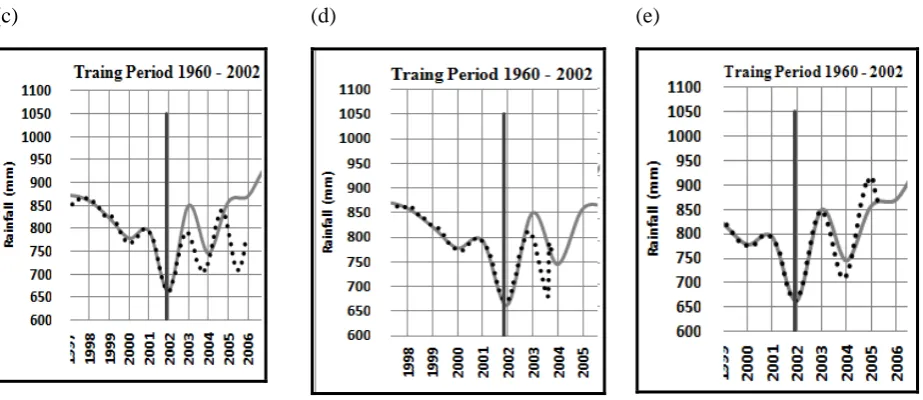
We have 51 input data samples as yearly average rainfall of 51 years, which is inadequate to support evaluation of a large prediction polynomial required for complex model like rainfall prediction. It is assumed that the desired prediction function is continuous and has no singularity. Data interpolation with higher order polynomial is achieved using .Net C# function DrawCurve() with tension values 0.5 as shown in Figure 1. This plots smooth curve containing 51 original data points on a bitmap object. The bitmap object contains a smooth curve containing 2001 points. These samples are extracted from bitmap object for virtually increasing the input sample size.
Figure 1 C# code sample for plotting continuous curve passing through discrete input points normData.
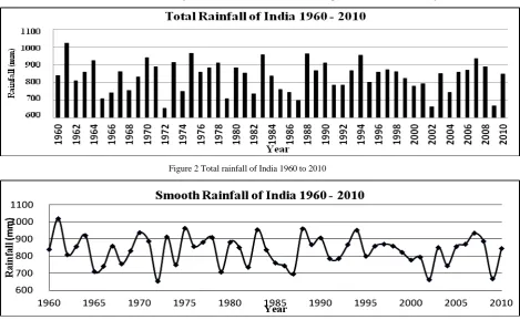
The actual rainfall of India is shown in Figure 2 The rainfall data after interpolation is shown in Figure 3
Figure 2 Total rainfall of India 1960 to 2010
Figure 3 India Rainfall data after smoothing
Prediction Model
The polynomial shown in eq. 1 is used as prediction algorithm in form of N×M matrix. The expression contains M previous rainfall samples to predict the next sample P(t+1). Each sample of forms Nth order polynomial with N coefficient Kn. Hence we have N×M values of to be evaluated to fit the rainfall
pattern.
for (int n = 0; n < normData.Length; n++) {
allPoints[n] = new Point(normData[n].Year, normData[n].Rainfall); }
Bitmap bmp = new Bitmap(2001, 1000); Graphics g = Graphics.FromImage(bmp);
1 1
The values of N and M are experimentally optimized to N = 11 and M = 20.
Here n is the order of polynomial and indicates the previous 20 points at interval of 10 samples.
Interpolated rainfall data points are at interval of ((51× 365)/2001) ≈ 9 days. This needs past (20×10×9) ≈1800 days data for prediction polynomial and this will predict the next rainfall value after (10×9) ≈ 90 days. The monsoon rainfall of India is for 3-4 months. To trace the trend within three months i.e. 90 days, each sample of M is considered at the interval of 10 data points. The year to year variation in rainfall is traced by M = 20 samples i.e. 1800 days. Based on these 1800 days model predicts the next 90 days ahead rainfall data. Prediction error tested outside training period is found less than 1%. The coefficient array K is derived by an iterative method to minimize the prediction error. The iterative method is evolved by defining error cost function and K is derived by minimizing the error cost function. The error cost function is defined as given in eq. (2)
1 1 … … … .2
Model Training
Model consists of M×N coefficients . A supervised training algorithm based on error gradient descendent technique is used to compute the values of all the coefficients. This is achieved by calculating the sensitivity of each coefficient with respect to prediction error.
Sensitivity is calculated as
1 1
1
1 … … … . .3
… … … 4Equation 4 shows the reinforcement of with learning rate
with value ranging from 0.001 to 0.01Where is the corrected value of the coefficient .To make the algorithm robust and noise tolerant we have added a small random noise to the final predicted value during training.
Regenerative Prediction Model
The above prediction model works successfully for prediction period of 90 days. A regenerative approach is used to extend the prediction period by including the predicted values in input stream. Like any other regenerative model also known as positive feedback, exhibits unstable behaviour. Stability is improved by training the model with regenerative loop. An extended prediction period of one year with less than 10 % error is achieved as shown in table I. The model predicts the rainfall of 90 days ahead by using previous 1800 days rainfall data. This predicted rainfall data is used as input in model for prediction of next value. The process is repeated using predicted data as new input. The average prediction error is 1% to 2% for 90 days and 2% to 10% for one year. This algorithm is implemented using interactive user friendly .Net C# tool and comma separated Excel text file format for input output file system. Rainfall prediction achieved for one year ahead is adequate period for crop planning in agriculture country like India.
III.RESULT AND DISCUSSION
The application is ported to Intel i3 CPU, @ 2.40 GHZ, with installed memory 3 GB laptop to evaluate the prediction algorithm. Two types of experiments conducted for model evaluation. (i) Open loop - In this method, input is used from the samples only, i.e. rainfall prediction is 90 days ahead. All the prediction results are for next sample i.e. 90 days with accuracy between 1 to 2 %. We have conducted approximate 150 experiments of this method. (ii) Close loop - In this method, model is evaluated using regenerative approach as mentioned above. 150 experiments are carried out. We present here top 10 results.
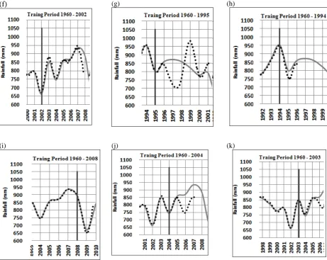
Figure 4(a)Unstable predicted trend in dotted line of test case-1, the regenerative model after few seconds.
The result is monitored interactively while training. Figure 4(a) and 4(b) shows the typical result of model for training period 1960 to 2002. In most training runs the predicted trend after few seconds showed unbounded unstable output as shown in Figure 4(a), however after few minutes of training the trend stabilizes within the acceptable limits as shown in Figure 4(b). The rainfall prediction error for 2003 is below 10%.
(b)
Figure 4 Comparison of actual and predicted rainfall for test case-1after 5 minutes of training.
(f) (g) (h)
(i) (j) (k)
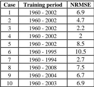
Figure 4(b) to Figure 4(k) shows the gray curve for actual and dotted curve for predicted rainfall results. In all the cases, model predicts the next one year rainfall with more than 90% accuracy. Table I and table II shows the numeric results for the different cases of actual and predicted rainfall with percentage error and normalized root mean square error. It can be seen that the error is below 10 % and the normalized root mean square error is between 2% to 10%.
Table I The actual and predicted rain fall values with prediction error.
Prediction for the Year
Actual Rainfall (mm)
Predicted Rainfall
(mm) Error % Error
1995 800.706 746.31473 54.39127 6.79
1996 858.437 876.42297 17.98597 2.1
1999 822.3551 842.62148 20.26638 2.46
2001 792.5876 774.80987 17.77773 2.24
2002 662.2417 653.01074 9.23096 1.39
2003 839.494 791.36171 48.13229 5.73
2004 748.3872 758.54183 10.15463 1.36
2005 857.535 899.49258 41.95758 4.89
2007 935.1111 886.33255 48.77855 5.22
2007 935.1111 872.8597 62.2514 6.66
2008 888.6556 859.18548 29.47012 3.32
Table II Normalized root mean square error for different cases.
Case Training period NRMSE 1 1960 - 2002 6.9
2 1960 - 2002 4.7
3 1960 - 2002 2.2
4 1960 - 2002 2
5 1960 - 2002 8.5
6 1960 - 1995 10.5
7 1960 - 1994 2.7
8 1960 - 2008 7.5
9 1960 - 2004 6.7
10 1960 - 2003 6.9
IV.CONCLUSION
The application developed using the proposed model is found as a useful interactive tool for prediction of Indian rainfall. The model is predicting more than one year rainfall trend with more than 90% accuracy. In average it predicts the quantity of rainfall one year ahead of time with reasonable accuracy which is help full for crop planning.
VI. REFERENCES
[1] Ajith Abraham, Ninan sajeeth Pjilip, Soft Computing Models for Weather Forecasting (2004), Journal of Applied Science and
Computations.
[2] A.A.Munot and K. Krishna Kumar, Long Range Prediction of Indian Summer Monsoon Rainfall – Indian institute of Tropical
Meteorology, Pune 411008, India (Feb-2007).
[3] Iyengar, R. N. and Raghukanth, S. T. G., Intrinsic mode functions and a strategy for forecasting Indian monsoon rainfall. Meteorol.
Atmos. Phys., 2004.
[4] M. Rajeevan, Prediction of Indian summer monsoon: Status, problems and prospects Special Section: Climate, Monsoon and India’s
Water Current Science, VOL. 81, NO. 11, 10 December 2001 1451.
[5] M. Rajeevan, D.S. Pai, R.AnilKumar, New Statistical Models for Long RangeForecasting of SouthWest Monsoon Rainfall over India,
NCC-Research Report, Indian Meteorological Department –Pune-411005, General of Meteorology (Research).
[6] K. Krishna Kumar , M. K. Soman and K. Rupa Kumar, Seasonal Forecasting of Indian Summer Monsoon Rainfall: A Review, IITM,
Pune, India, Weather, 50, 12, pp.449-467May 26, 2010.
[7] S. Karmakar, M. K. Kowar, P. Guhathakurta, Long-Range Monsoon Rainfall Pattern Recognition and Prediction for the Subdivision
'EPMB' Chhattisgarh Using Deterministic and Probabilistic Neural Network, 7th International conference on Advance in Pattern Recognition.
[8] Surajit Chattopadhyay, Goutami Chattopadhyay, Comparative study among different neural net learning algorithms applied to rainfall
time series, Meteorological Applications Volume 15, Issue 2, pages 273–280, June 2008.
[9] Sulochana Gadgil*, M. Rajeevan and Ravi Nanjundiah, Monsoon prediction – Why yet another failure?, CURRENT SCIENCE, VOL.
88, NO. 9, 10 MAY 2005.
[10] De Michele, C. and Bernardara, P. 2005, Spectral analysis and modeling of space-time. Atmospheric Research, pp. 124– 136.
[11] http://www.tropmet.res.in/ - Indian Institute of Tropical Meteorology, Pune
[12] Geoffrey E. Hinton Connectionist Learning Procedures, Computer Science Department, University of Toronto, 10 King’s College