Plant Modelling Framework: Software for building and running crop
models on the APSIM platform
*
Hamish E. Brown
a,*, Neil I. Huth
b, Dean P. Holzworth
b, Edmar I. Teixeira
a,
Rob F. Zyskowski
a, John N.G. Hargreaves
b, Derrick J. Moot
caThe New Zealand Institute for Plant&Food Research Limited, Private Bag 4604, Christchurch, New Zealand bCSIRO Ecosystem Sciences/Sustainable Agriculture Flagship, PO Box 102, 4350 Toowoomba, Australia cFaculty of Agriculture and Life Sciences, P.O. Box 85084, Lincoln University, 7647 Canterbury, New Zealand
a r t i c l e i n f o
Article history:
Received 30 September 2013 Received in revised form 1 July 2014
Accepted 3 September 2014 Available online 1 October 2014
Keywords: Canopy dynamics
Biomass and nitrogen partitioning Integrated design environment Phenological and morphological development
Reusable organ and function classes
a b s t r a c t
The Plant Modelling Framework (PMF) is a software framework for creating models that represent the plant components of farm system models in the agricultural production system simulator (APSIM). It is the next step in the evolution of generic crop templates for APSIM, building on software and science lessons from past versions and capitalising on new software approaches. The PMF contains a top-level Plant class that provides an interface with the APSIM model environment and controls the other clas-ses in the plant model. Other clasclas-ses include mid-level Organ, Phenology, Structure and Arbitrator clasclas-ses that represent specific elements or processes of the crop and sub-classes that the mid-level classes use to represent repeated data structures. It also contains low-level Function classes which represent generic mathematical, logical, procedural or reference code and provide values to the processes carried out by mid-level classes. A plant configurationfile specifies which mid-level and Function classes are to be included and how they are to be arranged and parameterised to represent a particular crop model. The PMF has an integrated design environment to allow plant models to be created visually. The aims of the PMF are to maximise code reuse and allowflexibility in the structure of models. Four examples are included to demonstrate theflexibility of application of the PMF; 1. Slurp, a simple model of the water use of a static crop, 2. Oat, an annual grain crop model with detailed growth, development and resource use processes, 3. Lucerne, perennial forage model with detailed growth, development and resource use processes, 4. Wheat, another detailed annual crop model constructed using an alternative set of organ and process classes. These examples show the PMF can be used to develop models of different com-plexities and allowsflexibility in the approach for implementing crop physiology concepts into model set up.
©2014 The Authors. Published by Elsevier Ltd. This is an open access article under the CC BY-NC-ND license (http://creativecommons.org/licenses/by-nc-nd/3.0/).
Availability
The Plant Modelling Framework source code is freely available for non commercial use and can be viewed at http://apsrunet. apsim.info/websvn/listing.php?repname¼apsim&path¼/trunk/ then clicking on the“Model”then“Plant2”folders. Note that the PMF (called Plant2 in internal documentation) does not stand alone and users will need to download the Agricultural Production Sys-tems Simulator (http://www.apsim.info/Products/Downloads. aspx) to build and use PMF models.
1. Introduction
A key purpose of APSIM is to simulate realistic long-term dy-namics in agricultural simulations (Holzworth et al., 2014; Keating et al., 2003). To do this, a range of arable, pasture, vegetable, tree, bush, vine and weed models are required to represent different kinds of plant communities and their contributions to the water and nutrient balance of agricultural land. However, the develop-ment and maintenance of many models requires considerable time andfinancial commitment. This problem is relevant to all agricul-tural systems modelling platforms that provide the capacity to simulate different crop types (Brisson et al., 2003; Jones et al., 2003; Stockle et al., 2003). Generic crop templates have been developed to address the problem (van Keulen et al., 1982;Penning de Vries
*Thematic Issue on Agricultural Systems Modeling&Software.
*Corresponding author. Tel.:þ64 3 325 9394.
E-mail address:[email protected](H.E. Brown).
Contents lists available atScienceDirect
Environmental Modelling & Software
j o u r n a l h o m e p a g e :w w w . e l s e v i e r . c o m / l o c a t e / e n v s o f t
http://dx.doi.org/10.1016/j.envsoft.2014.09.005
et al., 1989). They are based on the hypothesis that crop models can be constructed from a generic set of software classes that are then assembled and parameterised differently to represent the physi-ology of different crops. From this, the idea of process oriented programming was developed where sub routines represent a pro-cess defined as“a series of events, which drive the dynamics of the system in response to system attributes and environmental con-ditions” (Wang et al., 2003; Wang and Engel, 2000). A crop was defined as a system with a set of components such as phenology, organ genesis and biomass production. Processes are closely related to a specific system component and result in the change of the components state variables. Efforts have been made by a number of groups to increaseflexibility in the way that generic crop templates are set up to make models more adaptable to different requirements. The DSSAT group developed the CROPGRO template (Boote et al., 1998) in which crop coefficients are set in a‘species file’to configure the model as a particular crop type. CROPGRO has been applied to a large number of crops but has forced developers into afixed structure and numerous changes have been required to the code base to adapt it to different crop types. The APES simulator (Donatelli et al., 2010) provides a range of pre-determined crop model component options and parameters that the user selects through a graphical user interface (GUI). Similarly CROSPAL (Adam et al., 2010) provides a framework which combines expert knowl-edge and libraries containing crop modelling with a GUI that allows crop models to be assembled using combinations of different modelling approaches, However, to date CROSPAL based plant models have not been incorporated into a full farm systems model. Specific to the APSIM model,Wang et al. (2003)developed the generic crop model template (GCROP). This consisted of a set of component and function classes in a crop process library (source code) and configurationfiles. The configurationfile informed the APSIM model of what classes to assemble and what their parameter values were. This meant model developers could focus on deter-mining crop parameter values and evaluating crop models without the need to write model code. Reusing the same code for each model also meant maintenance was simplified because the code base was smaller and changes did not have to be repeated in multiple code sets whenever a fix or enhancement was imple-mented. In 2003 a new template was developed for APSIM which was derived from the ideas and structure of GCROP and the generic legume model (Robertson et al., 2002) implemented in Cþþand named PLANT in recognition of the application of the template to communities of plant species other that those defined as crops.
From the 41 plant models currently in APSIM (Holzworth et al., 2014), 26 are implemented using the PLANT or GCROP templates including cereals (Keating et al., 2001; Manschadi et al., 2006; Peake et al., 2008), legumes (Robertson and Carberry, 1998; Robertson et al., 2002; Turpin et al., 2003), horticultural crops (Robertson et al., 2002), vines (Huth et al., 2009; Robertson et al., 2005), pastures (Dolling et al., 2005; Probert et al., 1998b; Verburg et al., 2007) and weeds (Thornby et al., 2006; Whish et al., 2002). However, over time a number of limitations have been exposed in the PLANT template approach. In particular, it has a limited set of functionality available to model developers and creating new functions is difficult due to the structure and imple-mentation of the template. This has forced models into a fixed structure. However, different researchers have different, but equally acceptable, ideas about how reality should be abstracted. For instance, if data describing environmental responses are limited and the intended scope of model application is limited to specific situations (e.g. the study of yield under irrigated conditions at a single location), a simple model might be preferred. If the physi-ology of crop has been intensively studied and a model is to be used in a number of different situations (e.g studying yield, water and
nitrogen balance in a range of locations and management systems), a more detailed crop model will be preferred. Both approaches are legitimate in certain circumstances. As a result of the prescribed form of the generic template, crop modellers who want to take different approaches have not used it. Instead they have integrated alternative models into APSIM, resulting in contrasting code bases for crop models and a maintenance burden for the software team. New developments in the software industry (David et al., 2013), as well as lessons learned over the last 10 years from building models in the GCROP and PLANT templates (Holzworth and Huth, 2009b; Holzworth et al., 2010), have made an update to the generic crop template possible. Newer computer programming languages (e.g. C#) have the ability to inspect source code at run-time, extracting metadata about the code. This ability, called reflection or introspection (Rahman et al., 2004), can be used by a model framework to locate required functionality (classes) and determine their data requirements (inputs). This means that classes can be developed independently and models can be constructed at run time from executable mark-up language (XML)files that specify how to assemble and parameterise classes. The updated template is called the Plant Modelling Framework (PMF). This has been in development over the past 3 years aiming to achieve a number of key design goals:
Enable models to be established at different levels of
complexity.
Enable code reuse and minimise the amount of code to
maintain.
Externalise the structure and parameterisation of a crop model.
Provide a framework that enables the easy inclusion of new organ, process and function class alternatives.
The aim of this paper is to describe the PMF both conceptually and technically as a modular framework for building crop models and provide a set of example models of contrasting complexity to demonstrate its application andflexibility. One of these models is fully validated and previously implemented in APSIM (Wheat), one is a simple model also previously implemented in APSIM (Slurp) and two are alternatives to current APSIM models and still under development (Oat and Lucerne). This paper is not intending to provide a full description of these example models but use them to demonstrate different ways that science is translated into software in the PMF.
2. Description of the Plant Modelling Framework
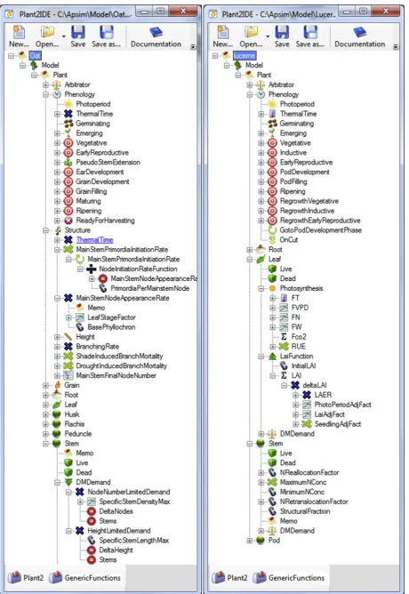
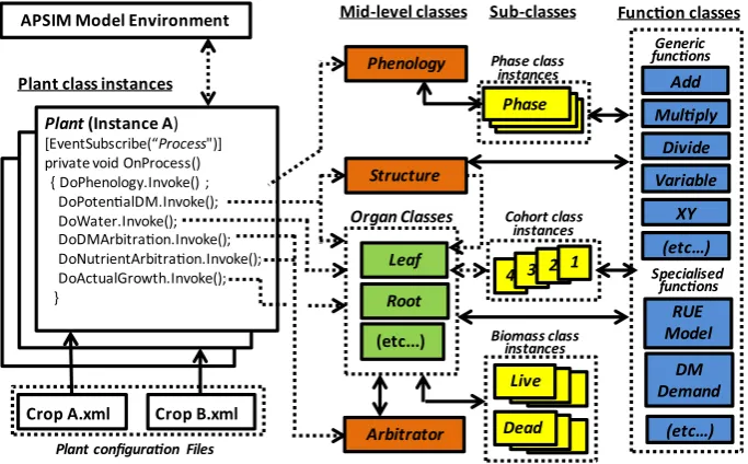
The PMF classes are abstracted at the plant or sub-plant level. However, an instance of PMF represents a community of identical plants so the basic units for class properties are expressed on an area basis (m2). Italics are used when referring to the names of specific classes, properties, events and values within the PMF software and names that refer specifically to the examples shown inFig. 1are given in single quotes. There are three main types of classes in the PMF (Fig. 2):
Top-levelPlantclasswhich provides an interface between in-stances of the crop model and the other models in the APSIM environment such as soil models and weather data. It also serves as an interface with the other PMF classes.
Mid-level classes.
that organ. These includeRoot,Leaf, ReproductiveandGeneric organ classes.
BProcess classes that orchestrate activity at the plant level and provide cues or instructions to organ classes. These include the arbitration of resource allocation to organs (Arbitrator class) and the phasic (Phenology class) and morphological (Structureclass) development of the crop.
BSub-classesthat organ and process classes delegate to for processes and/or data structures that repeat the same pattern. Multiple instances of a sub-class are used to repre-sent each repetition (e.g. live and dead biomass, phases of development, cohorts of leaves).
Low-level function classes contain generic mathematical, logical, reference or procedural code to return values to be used in mid-level class calculations.
Processes are programmed in a general way within the source code of mid-level classes. An example is shown in Fig. 3for the Structureclass. This class has a property ofMainStemNodeNowho's value is calculated daily in theDoPotentialDMevent method. The values for ThermalTime and MSNAppRatewhich are used in this calculation are links toFunctionclasses rather than simplefloating point declarations. The PMF infrastructure will look for aFunction with the same name as the declaration e.g. ThermalTime and MainStemNodeAppearanceRate.This allows any type of function to be selected providing the names match. Therefore, the model developer can chose different functions to provide values to the source code depending on how they want to represent it in their model. There are a range of broadly generic function classes that are used to implement a specific algorithm that can be used by many higher level classes (Table 1). There are also a number of specialised function classes that perform a single function, such as calculating an organ'sDMdemand, but are still generic as they can be re-used by any organ and any plant model. Function classes can also take the values they require from other function classes. Therefore,
functions can be assembled in many different ways to derive values for the processes contained in mid-level classes.
The type, arrangement and parameterisation of classes to be included in a model is specified by a plant configuration file (executable mark up language) and the PMF has an Integrated Development Environment (IDE) to allow plant models to be con-structed visually (Fig. 1). An example of how functions can be assembled to deliver values can be seen inFig. 1where the Oat ‘Stem’ Organ class calculates its ‘DMDemand’ using a Minimum function (‘DMDemand’). This gets its values from two Multiply functions (‘NodeNumberLimitedDemand’ and ‘ HeightLimitedDe-mand’) which in turn get their values from LinearInterpolation (‘SpecificStemDensityMax’), Constant (‘SpecificStemLengthMax’) and VariableReference functions (‘DeltaNodes’, ‘DeltaHeight’ and
Fig. 2.Schematic of the Plant Modelling Framework. Class types in the PMF source code include: the top level plant class which interfaces with the model environment, organ
classes (green shaded boxes), process classes (orange boxes), sub-classes (yellow boxes) that contain repeatable sub-sets of specific aspects of organ and process classes, function
classes (blue shading) that contain mathematical, procedural, logical or reference code to provide values to the other classes. Arrows show the direction of communications. (For
interpretation of the references to colour in thisfigure legend, the reader is referred to the web version of this article.)
Fig. 3.Example of selected source code fragments to demonstrate how mid level
‘Stems’). While functions that deliver values to a mid-level class have to have a name that matches the source code (‘DMDemand’in the example above), the names of subordinate functions are arbi-trary so they can be given names appropriate for the concept they represent (eg, ‘DeltaNodes’, ‘DeltaHeight’ and ‘Stems’ in the example above).
The Plant and lower level class structure and the use of a configurationfile to select and parameterise classes was also used in the original APSIM PLANT template. The additional structuring of classes into mid and low level classes and the development of an IDE for visual configuration is new to PMF.
2.1. Communications and process propagation
Instances of crop models communicate with the APSIM model environment using .NET events which are raised to correspond with management or processing events such asSow,Process, Har-vest,EndCropandCut(Moore et al., 2007). TheSowevent handler is invoked whenever a crop is to be sown. On this event the crop model constructs and configures its class hierarchy. The bulk of PMF computation is triggered by theProcessevent. In response to this event, thePlantclass raises a number of its own events (Fig. 2) that propagate processes through the mid-level classes:
1. DoPhenologyis subscribed to by thePhenologyclass and triggers calculation of daily crop development.
2. DoPotentialGrowthis subscribed to by the Structureclass and eachOrgan classes and triggers the calculation of how much
each organs number of constituents, dimensions and mass could change and how much DM and N they may contribute to plant growth.
3.DoWateris subscribed to byRootand Leaforgan classes and triggers calculations of water supply and demand used to determine the extent of water stress.
4.DoArbitratoris subscribed to by theArbitratorclass and triggers procedures to determine how much DM and N eachOrganclass will actually contribute and receive.
5.DoActualGrowth is subscribed to by Organ classes, triggering updates of other state variables and moves senesced biomass fromLivetoDeadbiomass pools.
Propagating processes through the PMF in this way enables flexibility of model structure. If a particular functionality is required, the appropriate class is included and responds to the appropriate events. If that functionality is not required in the crop model the class can be excluded from the configuration and the events that it would have responded to go unheard.
2.2. Phenology
Phenology is the development of crop through a series of phases which exhibit differences in the genesis of organs, nature or envi-ronmental response or resource partitioning. Crops differ widely in both the number of phases they contain and the types of behaviour exhibited within these phases. Similarly, model developers differ in their opinion of the number and type of stages that characterise crop phenological development. Phenology may not be required for simple crop models (such as Slurp) that do not change their func-tion over time. When phenology is required in a crop model, it is represented by including thePhenologyclass in the plant confi gu-rationfile with the necessaryPhasesub-classes (Fig. 1). The number and type of Phasesub-classes (Fig. 2) is unlimited by the source code and is at the complete discretion of the model developer. Phenology works on a daily time-step. Each day (when the DoPhenologyevent is invoked) thePhenologyclass interrogates the currentPhaseclass to determine if it has reached itsTarget. When it has, it calculates the proportion of the day that was not used to complete that phase and passes it to the nextPhaseclass instance. This is repeated each day until all phases have been completed. Rewind actions can also be included to return the crops develop-ment to an earlier phase to simulate the effects of defoliation on perennial crops. This structure enables phenology of varying de-grees of complexity to be established (Fig. 1). There are a range of Phasesub-classes representing different types of phenology which are described inTable 2and examples of the parameterisation of phases are given in Section3.
2.3. Structure
The Structure class represents the crops morphology and is required for models where organ classes need this information. The main properties of the Structure class include PlantPopulation, MainStemNumberPerPlant, MainStemPrimordiaNumber, Main-StemNodeNumber,MainStemBranchNumberandHeight.
2.4. Organs
All organ classes use the sameBiomasssub-class to keep track of their live and dead biomass status (Fig. 2). TheBiomasssub-class currently deals with DM and N content of organs. In the future it will also deal with P, K and other nutrients. Each of these compo-nents of biomass are separated into three types of pools repre-sented by the properties:
Table 1
Examples of function classes within the Plant Modelling Framework. Icons
corre-spond with functions shown inFig. 1.
Function type
Function name Return value
Mathematical Add Sum of all child class values
Subtract First child class value less all others
Multiply Product of all child class values
Divide The 1st child class value divided
by the 2nd
Exponential Ygivenxvariable and a, b, c coefficients
Sigmoid Ygivenxvariable and a, b, c coefficients
Power Ygivenxvariable and exponent
coefficient
Expression Parse and solve any expression
for givenxvariable.
LinearInterpolation Ygivenxycoordinates andxvariable
Constant Singlefixed value
Logical Maximum Maximum of all child function values
Minimum Minimum of all child function values
LessThan If variable reference<criteria return
child 1 value, else return child 2 value
GreaterThan If variable reference>criteria return
child 1 value, else return child 2 value
Reference Variable Value of specific PMF class property
ExternalVariable Value of specific property in
APSIM environment
DayLength Day length from latitude
and day or year
Procedural OnEvent Value 1 prior to event and
Value 2 after event
PhaseLookup Value of child function associated
with each phenological phase
Age Days since sowing
StructuralDMandNare essential for the growth of the organ. They remain within the organ once it has been allocated and are passed fromLivetoDeadpools as the organ senesces.
MetabolicDM and N are essential for growth and their con-centration can influence the function of organs (e.g. photo-synthetic efficiency of the leaf depends onMetabolicNcontent). MetabolicDM and MetabolicN may be reallocated (moved to another organ upon senescence of this organ) or retranslocated (moved to another organ at any time when supplies do not meet the structural and metabolic DM demands of growing organs).
NonStructuralDMandNare non-essential to the function of an organ. They will be allocated to an organ only when all other organs have received theirStructuralandMetabolicallocations and may be reallocated or retranslocated.
A range of organ classes have been developed for the PMF. The simplest is theGenericOrganwhich contains properties of biomass status and daily biomass demand and supplies (Table 3). The reproductive organ is similar to the generic organ but determines its biomass demands in a different way and also has aGrainNumber property.SimpleLeafandRootorgans deal with biomass demands the same asGenericOrgan. However,SimpleLeafincludes properties for DMSupply (photosynthesis), LeafAreaIndex, GreenCover and WaterDemand(Table 3). It is called simple because it is much less dynamic that the regularLeaforgan. TheRootorgan has additional properties ofDepth,RootLengthDensity, NSupply and WaterSupply. More detail of the different way these organs can be set up is given in Section3.
A phytomer typeLeafclass has also been developed for the PMF. It has the same basic properties asSimpleLeafbut predicts the area and biomass as the tally of areas and biomass of separate cohorts of leaves. A cohort of leaves is represented by a main-stem node po-sition and branch leaves are kept in the same cohort as the
main-stem leaf appearing at the same time (Lawless et al., 2005). The Leafclass delegates the status and function of individual cohorts intoLeafCohortsub-classes (Fig. 2). Further detail of theLeafclass is given in Oat model example below.
2.5. Biomass partitioning
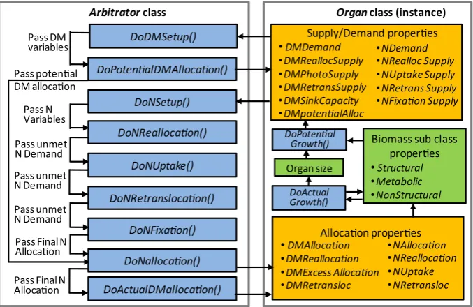
Organ classes have been designed around an arbitrator interface that provides a core set of properties thatOrganclasses may need to provide to the Arbitrator class with their biomass supplies and demands and to receive biomass allocations from theArbitrator (Fig. 4):
Table 3
Examples of Oragn classes in the Plant Modelling Framework including some of their key properties and the a brief description of the source code procedure associated with the computation of each property. Icons correspond with organs shown in
Fig. 1.
Organ class Properties Associated source code procedure
Generic Biomass Add N and DM types allocated
by the arbitrator and remove senescence calculated from SenescenceRate
StructuralDMDemand ReturnStructuralDMDemand
Function value NonStructuralDMDemand Return product of
StructuralDMFractionand StructuralDMless current NonStructuralDM
StructuralNdemand Return product of
MinimumNConcand StructualDMDemand
NonStructuralNDemand Return product of
MaximumNConcand current DM less current N
NReallocationSupply Return product of
ReallocationFactorandNSenescence calculated for that day.
NRetranslocationSupply Return product of
RetranslocationFactorand
currentNonStructuralN.
Reproductive GrainNumber Return GrainNumber
function value
StructuralDMDemand PotentialDMFillingRate
MaximumGrainSize1
StructuralNdemand PotentialNFillingrate
MinimumNConc
MaximumNConc1
GrainNumber
Simple leaf Biomass properties As for generic organ
DMSupply Return value ofPhotosynthesis
function
LeafAreaIndex ReturnLAIfunctionvalue
GreenCover ReturnGreenCover
WaterDemand Return Transpiration demand
calculated by micro-metrological
component2
Root Biomass properties As for generic organ
Depth Add dailyRootExtnesionRatevalue
to current depth3
NSupply Obtains extractable mineral N from
each soil layer within rootDepth4
WaterSupply Obtains extractable soil water from
each soil layer within rootDepth5
References.1Asseng et al. (2002).2Snow and Huth (2004).3Robertson et al. (1993).
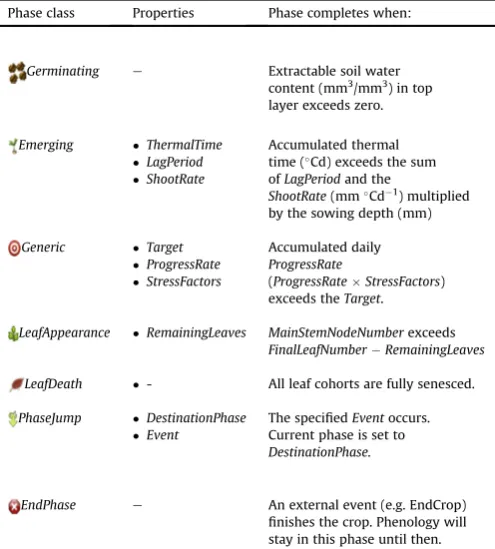
4Probert et al. (1998a).5Meinke et al. (1993). Table 2
Description of phase sub-classes used to construct phenology in the PMF. Icons
correspond with phases shown inFig. 1.
Phase class Properties Phase completes when:
Germinating e Extractable soil water
content (mm3/mm3) in top
layer exceeds zero.
Emerging ThermalTime
LagPeriod
ShootRate
Accumulated thermal
time (Cd) exceeds the sum
ofLagPeriodand the
ShootRate(mmCd1) multiplied
by the sowing depth (mm)
Generic Target
ProgressRate
StressFactors
Accumulated daily ProgressRate
(ProgressRateStressFactors)
exceeds theTarget.
LeafAppearance RemainingLeaves MainStemNodeNumberexceeds FinalLeafNumberRemainingLeaves
LeafDeath - All leaf cohorts are fully senesced.
PhaseJump DestinationPhase
Event
The specifiedEventoccurs.
Current phase is set to DestinationPhase.
EndPhase e An external event (e.g. EndCrop)
finishes the crop. Phenology will
Biomass supply and demand properties, which are set by each organ class and interrogated by theArbitratorclass:
BDMSupply contains supply types Photosynthesis, Retrans-locationandReallocation
BDMDemand contains types Structural, Metabolic and NonStructural
BDMPotentialAllocation contains types Structural, Metabolic and NonStructural which are used to calculate NDemand types
BNSupplycontains supply typesReallocation, Uptake, Fixation and Retranslocation
BNDemandcontainingStructural, MetabolicandNonStructural types.
Biomass allocation properties that are set by theArbitratorclass to deliver biomass allocations to each organ class:
BDMAllocation containsAllocation, Reallocation and Retrans-locationtypes
BNAllocationcontainsAllocation, Reallocation, Uptake, Fixation andRetranslocationtypes.
To minimise the amount of code needed, these arbitrator interface properties are all contained within aBaseOrganclass and all other organ classes inherit from this. Each property has zero values by default and code written into the appropriate properties of inheritingorganclasses overwrites these defaults. Specific organ classes only contain procedures to assign values to those supplies and demands that are relevant. For instance the Leaf class is currently the only one that contains aPhotosynthesisDMSupplyand theRootclass is the only one containing anUptakeNSupply. How-ever, if models require other organs to photosynthesise or take up N, these can be added into otherOrganclasses without needing to reengineer the arbitrator interface.
The Arbitrator regulates the partitioning of biomass among Organs using resource supplies and demands from each Organ instance (Fig. 4). The growth of a plants DM is the minimum of DM supply from photosynthesis and DM demands from struc-tural growth and the capacity to store non-strucstruc-tural DM (Gent and Seginer, 2012). The PMF arbitrator extends this idea to the organ scale where the DM supply becomes that of photosyn-thesis plus the reallocation and remobilisation of non-structural DM from other organs. In situations where DM demands exceed supplies theArbitratorclass can partition to organs based on their demand relative to other organs or on a user-specified priority ranking. The partitioning of N is inherently linked to DM partitioning in the PMFArbitratorclass based on the parti-tioning concepts of the SIRIUS modelling approach (Jamieson et al., 1998).
ThePlantclassfirst invokesDoPotentialGrowth(Fig. 2) when each organ determines how much its biomass, dimensions and number properties could increase and sets the values of DMSupply and Demand properties (Fig. 4). Next it calls DoD-MArbitration and DoNArbitration which trigger a sequence of functions in theArbitratorclass to determine how much DM and N will be allocated to each organ (Fig. 4).DoPotentialDMAllocation takes PhotosynthesisDMSupply and ReallocationDMSupply, parti-tions these to organs based on their Structural and Metabol-icDMDemands and partitions any SurplusDMSupply to organs based on their NonStructuralDM demand. If someDMSupply is still unallocated this remains unallocated with the assumption that the plant would down regulate photosynthesis due to lack of sink capacity in such cases (Gent and Seginer, 2012). If the Structural and MetabolicDMDemand are not met Retrans-locationDMSupply is used to meet these demands. Then DoN-Reallocation, DoNUptake, DoNRetranslocation, and DoNFixation determine organNAllocationfrom each of these supplies. DoAc-tualDMAllocationtakesNAllocationsfor each organ, determines if this is enough to maintainMinNConcand if not theDMAllocation is constrained andSurplusDMdiscarded. This assumes that under severe N stress photosynthesis would be down regulated due to N inadequacy limiting sink strength (Gent and Seginer, 2012; Jamieson et al., 1998).
Fig. 4.Schematic showing procedure for biomass partitioning arbitration. Orange boxes contain properties that make up the organ/arbitrator interface. Green boxes are organ
specific properties and blue boxes contain events which are triggered during the daily time step of the model. (For interpretation of the references to colour in thisfigure legend, the
Currently arbitration has only been implemented to deal with N supply. However, P, K and other nutrients can also be included in the same way with each organ registering supplies and de-mands, the arbitrator allocating these and constraining DM al-locations to maintain minimum nutrient concentrations in organs.
2.6. Water stress responses
Water stress is represented in PMF using a
Water-SupplyDemandRatioproperty calculated as supply/demand (Brown et al., 2009; Wang et al., 2004). The supply comes from theRoot organ (Table 3) and demand from the MicroMet model in APSIM (Snow and Huth, 2004). Values1 mean water supply is able to met demand and values<1 infer some degree of stress. Processes that are influenced by water stress have their rates multiplied by stress factors. The PMF allows water stress factors to be included to influence any process. Currently they are applied to photosyn-thesis, leaf area expansion, stem extension, leaf senescence, branch mortality and N fixation. These responses to water stress are configured in the crop.xmlfiles (e.g. the‘FW’function under ‘Photosynthesis’in the‘Leaf’organ of the lucerne model,Fig. 1).
3. Crop model examples
3.1. Slurp
The simplest crop model implemented in PMF is Slurp (named after the action of slurping water from the soil) which consists of SimpleLeafandRootorgans. This model is for the purpose of doing water balance studies where detailed representation of plant pro-cesses are not required, e.g.Snow et al. (2007). The functionality given byArbitrator,PhenologyandStructureclasses is not needed so these classes are omitted from the Slurp configuration. The values ofLeafAreaIndex,HeightandRootDepthare given toLeafandRoot organs byConstantfunctions.
3.2. Oat
The oat model is an example of a complex crop model, currently under development, to demonstrate the functionality of the cohort leaf class.
3.2.1. Phenology
The structure of the phenology model is displayed inFig. 1. The ‘Germinating’ phase is represented by aGerminationphase class and the‘Emerging’phase by anEmergingphase class (Table 2). The emergence phase leads into a‘Vegetative’phase which is currently represented by aGenericphase class (Table 2) with a constant 70C ThermalTimeTarget. This can be expanded with more detailed functionality in the future to represent vernalization responses of sensitive cultivars. Next is the‘EarlyReproductive’phase, which is also aGenericPhaseclass with aThermaltimeTargetthat uses a Lin-earInterpolationfunction to decrease from 650Cd to 400Cd, as photoperiod increases from 10 to 16 h. This captures the photo-period sensitivity that is displayed by oats (Martin et al., 1998a). FinalMainStemNodeNumber is set in the Structure class on the completion of the early reproductive phase (Section2.3) and the following‘PseudoStemExtension’phase is aLeafAppearancephase class (Table 2) thatfinishes whenflag leaf has appeared. Following this there are a series ofGenericphase sub-classes withConstants for ThermaltimeTarget representing grain development and ripening phases (Fig. 1).
3.2.2. Structure
In the oat model MainStemPrimordiaNumber is assumed to represent the number of primordia committed to becoming leaves. In cereals the commitment of primordia to becoming leaves in-creases as a linear function of leaf appearance untilfloral initiation, when the fate of all primordia is set (Brown et al., 2013; Jamieson et al., 2007). Sonego et al. (2000)showed that final main-stem node number in‘Drummond’oats is related to the modified Haun stage at whichfloral initiation occurs (FIHS) by:
FinalMainStemNodeNumber¼2:8þ 1:2FIHS
To model this,MainStemPrimordiaNumberis set to 3 at the time of emergence andMainStemPrimordiaInitiationRateis calculated by dividing MainStemNodeAppearanceRate by 1.2 (‘ Primordia-PerMainstemNode’function inFig. 1).MainStemPrimordiaNumberis fixed atfloral initiation (the end of the‘EarlyReproductive’phase)
which determines the upper limit for MainStemNodeNumber
(Fig. 5a). Thus, the photoperiod response that is programmed into
the early reproductive phase directly affects
Final-MainStemNodeNumberand the timing offlag leaf and subsequent anthesis (Section3.2.1). The value ofMainStemNodeAppearanceRate for predicting MainStemNodeNumber (Fig. 5a) is delivered by a Multiplyfunction (‘MainStemNodeAppearanceRate’inFig. 1) that provides the product of‘BasePhyllochron’(Constantfunction) and ‘LeafStageFactor’ (LinearInterpolation function) that decreases as MainStemNodeNumber increases (Jamieson et al., 1995; Martin et al., 1998b).
The‘BranchingRate’(number of new branches produced each day,Fig. 1) is given by aMultiplyfunction that returns the product of a ‘PotentialBranchingRate’, a ‘ShadingFactor’ and a ‘ Water-StressFactor’. In oats, thefirst tiller appears when the 4th main-stem node appears and in wide spaced plants a further tiller may appear with each main-stem node untilfloral initiation. To repro-duce this process the PotentialBranchingRate is aPhaseBasedLookup function with a LinearInterpolation function returning a value (increasing from 0 for the first 3 main-stem nodes, to 1 for all subsequent nodes) from emergence until floral initiation and returning aConstantof zero for subsequent phases. As plant spacing decreases the extent of tillering on individual plants decreases also. To capture this, the‘ShadingFactor’is aLinearInterpolationfunction which has a value of 1.0 whenGreenCover is between 0 and 0.5, decreasing to 0 at aGreenCoverof 0.8. This means, at lower ulations, plants will produce more tillers than at higher
pop-ulations. ‘ShadeInducedBranchMortality’ and
‘DroughtInducedBranchMortality’ functions are also included (Fig. 1) withLinerInterpolationfunctions returning positive values at highGreenCoverand lowWaterSupplyDemandRatiorespectively.
3.2.3. Leaf organ
whenOverlyingCoverexceeds 0.97. Thus, when a crop has a high stem population and many leaves, the lower leaves will senesce away keepingLeafAreaIndexat realistic values. A comparison of the size of each leaf position relative to that predicted for each cohort is shown inFig. 5b and the net LeafAreaIndex predicted from this model for different drought treatments shown inFig. 5d.
3.2.4. Other organs
The‘Grain’in the oat model (Fig. 1) is represented by a Repro-ductiveorgan class (Table 3). TheGrainNumbergiven by aMultiply function which returns the product ofStructure.TotalStemPopulation (using aVariableReference function), the number of ‘ PaniclesPer-Stem’(aConstantof 0.83), the number of‘SpikeletsPerPanicle’(a Constantof 25) and the number of‘GrainsPerSpikelet’ (a Linear-Interpolationreturning a value which increases from 0 atflowering up to 1.95, 250Cd afterflowering).
The‘Stem’is represented by theGenericOrganclass (Table 3). Stem weight is correlated with node number (main-stem and branched nodes) over a range of water stress conditions giving differences in internode length (Martin, unpublished data). This shows there is plasticity in the specific length (mm g1) of nodes so when stress reduces node expansion the nodes can become denser. However, under severe stress the correlation between node num-ber and stem mass changes suggesting there is a limitation to how dense internodes can become. To capture this, the Structur-alDMDemand is determined using a Minimum function which returns the lowest of‘DeltaNodeNumber’and‘DeltaHeight’limited demands (Fig. 1). The‘Husk’,‘Rachis’and‘Peduncle’organs are also
represented by the GenericOrgan class but with simple
representations of StructuralDMDemand using a function class called PopulationBasedDemand. This function has parameters of MaximumOrganSize,StartStageandGrowthDuration. Linear growth is assumed so dailyStructuralDMDemandof each organ is calculated as the product of PotentialDailyGrowth (MaximumOrganSize/ GrowthDuration), ThermalTime, aWaterStressFactorand the Total-StemPopulation(assuming each stem has one of these organs). An example of the biomass accumulation patterns that result from these organ class parameterisations is shown inFig. 5c.
3.3. Lucerne
Lucerne is a perennial crop that is frequently cut and the extent of biomass partitioning to below ground organs varies among the consecutive regrowth periods throughout the year (Teixeira et al., 2007a). It is also a crop for which recent advances in physiology had been included into another model (Teixeira et al., 2009). The lucerne model is used to demonstrate how feasible it is to repro-duce the functionality of an alternative model of intermediary complexity into PMF.
3.3.1. Phenology
TheGermination, Emerging,andGeneric Phaseclasses (Table 2) are used to construct the development of the lucerne crop from sowing e harvest ripe (Fig. 1) with phases parameterised as described byTeixeira et al. (2011). Lucerne differs from the other crop models described because it is perennial (as opposed to annual) and regrowth must be modelled. To achieve this there are a set of regrowth phases that the crop proceeds into once grain
1-Oct 1-Dec 1-Feb 1-Apr
Numb
er
0 2 4 6 8 10
1-Oct 1-Dec 1-Feb 1-Apr
Leaf
Siz
e
(cm
2 )
0 10 20 30 40 50 60
Veg etat
ive Prim
ordi a
Sene sced
coho rts
Exp ande
dco horts
App eare
dC ohort
s
1-Oct 1-Dec 1-Feb 1-Apr
Lea
f area
index (m
2 m -2 )
0 2 4 6 8 10
Late Full Nil Early
1-Oct 1-Dec 1-Feb 1-Apr
We
ig
ht
(
g
m
-2 )
0 200 400 600 800 1000
Stem Leaf Grain Husk Rachis
a b
c d
Fig. 5.Oat model predictions compared with observations for a) the initiation of primordia (when cohorts are initialised), the appearance of that cohort and the completion of its
expansion and senescence; b) the expansion and senescence of leaves at subsequent main stem positions; c) the growth of organs; d) the leaf area index of treatments receiving
production is complete (Fig. 1). The crop will also reset phenology to the‘RegrowthVegetative’phase each time a defoliation event is specified by the APSIM Manager module. When regrowth reaches the end of the ‘RegrowthEarlyReproductive’phase, phenology is then re-set to the‘PodDevelopment’phase (Fig. 1) so the same phases can be used to represent the seedling and regrowth crop.
3.3.2. Leaf organ
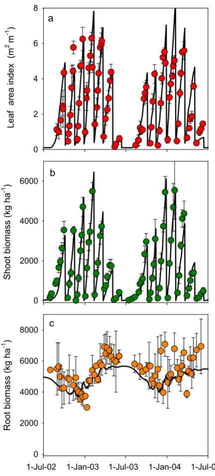
In the case of lucerne, the complexity of seasonal changes of leaf size and branching dynamics makes it challenging to parameterise the phytomer model in theLeafclass. Instead theSimpleLeafclass (Table 1) was used with functions included to provide changes in LeafAreaIndex, DMSupply and DMDemand (Fig. 1). Teixeira et al. (2007b)showed the daily increase inLeafAreaIndexof lucerne is closely related to thermal time in unstressed crops with Main-StemPopulation greater than 800 stems/m2. To capture this Leaf-AreaIndexis modelled using anAccumulatefunction (’LAI’inFig. 1) which keeps a tally of daily increments (‘DeltaLAI’) in response to ThermalTime. ‘DeltaLAI’ uses a Multiply function to return the product of (i) potential leaf area expansion rate (‘LAER’, aConstant value of 0.016 m2 leaf per m2 of soil per Cd), (ii) a ‘ Photo-PeriodAdjFact’(LinearInterpolationretuning a value of 1.0 for pho-toperiods> 12, reducing to 0 at a photoperiod of 10.0 h), (iii) a ‘LAIAdjFact’(LinearInterpolationfactor to reduce expansion rates at LAI<1) and (iv) a‘SeedlingAadjFact’which was aPhaseLookupclass returning a value of 0.6 for seedling phases and 1.0 for regrowth phases. TheAccumulateclass subtracts a specified proportion from value when a defoliation event is sent from the APSIM model so LAI is decreased in response to such events. The LAI model is relatively simple collection of functions but was able to reproduce the LAI dynamics of a lucerne crop for 2 years from sowing (Fig. 6a).
The ‘Leaf’ was as SimpleLeaf organ given a DMSupply by including theRUEModelfunction (‘Photosynthesis’inFig. 1) para-meterised using the RUE responses described by Brown et al. (2006). The ‘DMDemand’ for leaf was provided by including a PartitionFractionDemandfunction which returns a demand that is the product ofDMSupply and aPartitioningCoefficientwhich was adapted from the one described byTeixeira et al. (2009).
3.3.3. Stem and root organs
The‘Stem’organ used theGenericOrganclass (Table 3) with a PartitionFractionDemand function to set its ‘DMDemand’ as described by Teixeira et al. (2009). The tap andfine roots were represented with theRootorgan class which provides mineral N and water supplies to the arbitrator and keeps track of below ground biomass. Lucerne shows a seasonalfluctuation in below ground DM with increases in the autumn and reductions in winter and spring (Fig. 6c). This was modelled by using two collections of functions to reproduce seasonal patterns of (i) biomass partitioning to roots and (ii) root senescence plus maintenance respiration adapted fromTeixeira et al. (2009). This set up was able to repro-duce the complex seasonal patterns of shoot and root DM observed in a lucerne crop (Fig. 6) without requiring any changes to the source code ofRootorgan class.
3.3.4. Flexibility for further model development
This example shows that the PMF framework enabledflexibility to successfully implement a previously developed lucerne model (Teixeira et al., 2009) for crops growing under unconstrained water, nutrients and harvest management conditions. This basic set up enablesflexible expansion of the model capability. Specifically, to account for sub-optimal growth conditions, lucerne reserve organs (e.g. crowns and taproots) have to be implemented to store nitro-gen, a root nodule organ is required tofix atmospheric nitrogen and water stress responses have to be parameterised. This will enable
the model to deal with the effects of severe grazing on root biomass and shoot regrowth. In addition, the uncoupling of root respiration and senescence, the effects of low population on canopy growth, and inclusion of varieties with contrasting dormancies, as described in the existing version of APSIM, can be easily transferred to this pilot lucerne model.
3.4. Wheat model
Wheat was initially a series of translations of the CERES wheat model (Ritchie and Otter, 1985) into the Fortran77-based APSIM framework (Asseng et al., 1998; Keating et al., 2001; Meinke et al., 1997). Upon the development of the GCROP template (Wang et al., 2003), the science of these was translated into this generic
1-Jul-02 1-Jan-03 1-Jul-03 1-Jan-04 1-Jul-04
Root biomas
s (kg ha
-1
)
0 2000 4000 6000 8000
S
hoot biomass (k
g ha
-1
)
0 2000 4000 6000
Leaf
area index
(m
2
m
-1)
0 2 4 6 8
a
b
c
Fig. 6.Observations and predicted values of a) leaf area index; b) shoot biomass; and
c) root biomass of lucerne. Observed data fromTeixeira et al. (2007a)andTeixeira et al.
crop template which also represented a move to Fortran90. This was then merged into a code base which also allowed for simula-tion of legumes and perennial plants (Robertson et al., 2002) to make an even more generic modelling framework and represented another language move into C and then Cþþ. This model evolution has been driven by the advantages of moving to more generic de-signs, including object oriented and pattern-based development at each step. Science developments have been implemented into the model over this time also with most functionality being maintained from one version to the next. Ongoing testing (Holzworth et al., 2014, 2011) has ensured that model performance and integrity has been maintained during each evolutionary step. The docu-mentation of APSIM wheat is available online (www.apsim.info).
The decision was made to further evolve the wheat model into the PMF to make use of its better design. However, the wheat model was already extensively validated and has a large user base, and so it was important to ensure that model performance was main-tained. Whilst it is desirable to implement the wheat model using the PMF classes described above, doing this and re-testing the model would require a considerable effort. Processes are being developed to help accelerate these processes. However, until these become available, it was decided to conduct a software port of the existing wheat model into PMF by using PMF components wher-ever possible and porting other required processes into C#. It was possible to use the PMF phenology classes to represent develop-ment and capture much of the remaining functionality in function classes. The result is a set of new mid-level classes (Fig. 2) that replicate the existing wheat model.
The PMF Wheat model produces outputs that are identical to those of the existing wheat model in the standard APSIM wheat model validation set containing 164 simulations for a wide range of environments and treatments (Supplementary material). The pre-dicted yields for above ground biomass (Fig. 7a), grain yield (Fig. 7b), and nitrogen content in above ground biomass (Fig. 7c) and grain (Fig. 7d) all showed good agreement with observed values. These results show that this intermediate step in the model's evolution can still be used with confidence by the APSIM user community whilst we continue to move toward using more of the standard PMF classes.
4. Discussion
Plant models are undergoing continual evolution as progress is made in the science that they represent and the software that is used to implement them. The notion of a generic crop template has evolved as a means of improving the efficiency of development of models and maintenance of source code. However, some crop templates such as CROPGRO (Boote et al., 1998) GCROP (Wang et al., 2003) and PLANT (Robertson et al., 2002) have been overly pre-scriptive of the way models were structured and the data that is needed to represent them. Generic crop templates have also suf-fered from developers and maintainers not wanting to make changes to the source code to overcome a problem or expand the science for one crop for fear of affecting the performance of other crop models built using the same code base. The PMF is the next generation of crop template that attempts to achieve the same
Observed biomass (t ha-1)
0 5 10 15 20 25
Pre
d
ic
te
d Bi
omas
s (
t
ha
-1 )
0 5 10 15 20 25
Observed Grain Yield (t ha-1)
0 3 6 9 12
Pr
ed
ic
te
d Gr
ain
Y
ie
ld
(t ha
-1 )
0 3 6 9 12
Observed biomass N (kg ha-1)
0 100 200 300 400
Pr
edi
cte
d Biomas
s N
(k
g h
a
-1 )
0 100 200 300 400
Observed Grain N (kg ha-1)
0 100 200 300
Pr
ed
icted Gr
ai
n N (k
g
ha
-1 )
0 100 200 300 y = 0.95x + 1.04
R2 = 0.93
y = 0.93x + 0.28 R2 = 0.92
y = 0.88x + 21.95 R2 = 0.87
y = 0.91x + 10.33 R2 = 0.87
objectives as previous crop templates while providing morefl exi-bility in the way models are structured and reducing the need for model developers to write or compile code. A number of design goals were outlined in the introduction and in the sections below we consider how successful the PMF has been in achieving these:
4.1. Enable models to be established at different levels of complexity
Creating models with different levels of complexity was considered important so software developers were not limiting the approaches that crop physiologists and modellers could take in the development of crop models. Thisflexibility is achieved in three ways. Firstly by using afixed interface for the communication be-tween top and mid level organs (Fig. 1) without any mandatory mid-level classes allows functionality to be added or subtracted as needed. Secondly by providing a range of mid-level classes with different sets of functionality at different levels of detail (eg Sim-pleLeafvs phytomerLeafclasses) or with different approaches (e.g the Wheat model classes) allows the developer to choose an appropriate level of complexity. Thirdly, by programming the mid level classes generically, the developer can choose a combination of Function classes that matches the required level of complexity. (Section2). The examples given in this paper show models ranging from very simple (slurp), intermediate (lucerne) and detailed (oat and wheat) and all have been successfully implemented in PMF showing this design goal has been achieved. Thisflexibility is not unique to PMF with the APES model (Donatelli et al., 2010) also allowing models to be assembled at different levels of complexity. As the types and scale of applications for crop models broadens, modellers will require increasing flexibility in how models are structured and parameterised and it seems fair to expect that software developers must provide tools to enable thisflexibility.
4.2. Enable code reuse and minimise the amount of code to maintain
This is a key goal of all generic crop templates (Adam et al., 2012; Jones et al., 2001; Penning de Vries et al., 1989). The PMF classes represent generic elements of the plant structure or function and can be parameterised to represent different sets of functionality for different crops. For example, the oat model shown inFig. 1contains four instances of theGenericOrganclass (Husk, Rachis, Peduncle and Internodes). In each case, this class is parameterised differently to represent the different kinds of organs. The use of sub-classes to represent repeated data structures and processes as well as the extensive use of function classes also achieves code reuse each time a particular mathematical or procedural computation is made. At this stage we can conclude that PFM has achieved its goal of max-imising code reuse. However, as the number of developers using PFM increases it is likely that overlapping functionality will be written because those new to the system will not be fully aware that the current library of functions contains the mechanisms needed. This is a case for good documentation and easy visualisation of the available source code classes. Reflection tags allow for the inclusion of documentation within source code and the rendering of it using auto documentation systems which have been used to produce documentation of some PMF models. However there is also a need for a system to extract comments from the source code and asso-ciate them with classes in the IDE so instructions displayed there remain in sync with source code development.
4.3. Externalise the structure and parameterisation of a crop model
Externalisation of model structure and parameterisation (Holzworth and Huth, 2009a) eliminates the need for model
developers to compile source code. The PMF is facilitated by gen-eralising the classes and externalising the calculation of the values they use into function classes (Fig. 1). Thus, nearly all of models functionality is determined by which mid-level classes are included and how function classes are combined to provide their values. There are still large parts of the models functionality that are inherent to the structure of the source code within classes and their interfaces (such as the arbitration procedures) and cannot be changed without traditional coding and compiling. However, the PMF enables considerably moreflexibility to change models from the configurationfiles than previous crop templates allowing non-programming model developers moreflexibility than was previ-ously available. With the large number of functions and classes available, it can be daunting for new developers to achieve an un-derstanding of which parts to‘click’together when creating a new plant model. This is another case for developing good documen-tation and tools to ease the developer through this process.
4.4. Provide a framework that enables the easy inclusion of new organ, process and function class alternatives
The PMF contains a set of generic classes that have already been used to build a number of crop models. However, if a modeller wants to change some of the fundamental processes or properties of a class, alternative mid-level or function classes can be written and included in the source code (e.g. the Wheat model, Section3.4). If developers wish to aggregate processes in a different way, they can write alternative classes that interface with the plant class and use any of the function classes to provide them with values (e.g. the wheat model). This design conflicts with the goal of maximising code reuse because it allows for multiple ways of doing things. However, the need to enable alternative approaches is necessary to allow scientific exploration of modelling approaches and to make development in the PMF environment comfortable for a broad range of developers. The successful achievement of this design goal might contribute to enlargement of the source code and the maintenance burden for the software team. However, the low level function concept will help slow code enlargement and thefl exi-bility that this provides to model developers is seen as a worth-while benefit.
4.5. Potential problems and misuse of PMF
One possible problem is that making the model structure accessible to more developers is loss of control of the model code with the prospect of developers making unjustified changes to the model then representing it as the released version. The greater ease in setting up models could also encourage ill-informed model development. To partially address this issue we need to make it clear to would-be-developers that a detailed understanding crop physiology is an essential prerequisite to construction of a robust model in PMF (as it is for any model platform). We will also emphasise that best practice should always be followed in the use of models. Specifically, any changes that have been made to a released version of a model must always be clearly detailed and justified. Ultimately though, model performance will be judged by its validation against observed data. Like all major changes to models in APSIM, new or altered PMF models will be reviewed by the APSIM reference panel for scientific merrit, design and imple-mentation, before being included in official releases (Holzworth et al., 2014). This helps to minimise any potential misuses of the PMF.
general principal of PMF development is to write descriptive error messages whenever a fatal error or fundamental violation is iso-lated in debugging. The use of .NET also means that any variable can be reported, which facilitates the isolation of unexpected behaviour of a model component. While the IDE approach to developing models makes them accessible to non-programming developers, the XML representation of a plant model is itself a programming language that developers need to learn. For computer programmers familiar with other languages, this is sometimes viewed as limiting and inefficient and may discourage programmers from using PMF. The delegation of functionality into function configurations moves the code base from the compiled classes to the XMLfiles which means this code is not shared between models. Science ideas that are represented by a nest of functions can be copied from one model to another to share the science but this creates duplication of XML fragments in the plant configurationfiles potentially leading tofixes needing to be repeated across multiple sets offiles. To alleviate this, when a particular pattern of functions occurs in several configurationfiles, a specialised function is created repre-senting the algorithm and each configurationfile is changed to use the new function.
One problem that has hindered past crop templates is the inherent desire to minimise changing code once it provides the basis for validated models. This limits the scope for allowing bug fixes or code improvements to aid other models that use the same code base. The delegation of model structure into plant confi gu-rationfiles solves this problem to a certain extent but there is still structure in the source code. To ensure the code base of PMF was not dictated by thefirst few models produced, its development to date has not focused on completing and validating crop models. Instead the focus has been on the establishment of a wide range of models to test the generic applicability of the code base, work out any bugs and develop software methods that will enable changes to one model without adversely affecting the performance of another. As such, a number of models have been established in PMF including Oat, Lucerne, Potato (Brown et al., 2011), Field Pea, Kale, Barley, Grape, E.Grandis, Chickpea, Broccoli (Huth et al., 2009), French Bean, Wheat and OilPlam (Huth et al., in this issue).
4.6. Future development
Now that the code base is reaching a point of stability, the focus will move onto the completion of some of these models and the migration of existing APSIM crop models into the PMF. To achieve this some work is still required to reconcile the alternative ap-proaches taken in the arbitration of DM and N allocation in PLANT and the PMF. The process of migration could also be accelerated by including a LeafAreaIndex function for the SimpleLeaf organ (Table 3) that is analogous to that used in the PLANT template. This will mean migration will not need to involve the parameterisation of a completely new canopy model (Table 3).
The PMF has been moved into the next generation of APSIM (Holzworth et al., 2014) and will form the basis of many new and upgraded models of the plant based components of the APSIM model. This new generation of APSIM will offer an improved model validation and testing procedure. In combination with the ease of model development in the PMF, this will enable faster progress improving the science content and reliability of APSIM crop models. Functionality that will be added to the PMF over the next few years includes the ability to simulate multi species crops. To do this a separate component is being developed to arbitrate inter-plant resource allocation. It will interface with multiple instances of PMF models and provide them with their portion of the daily ra-diation, water and nitrogen they can obtain for their daily pro-cesses. Another feature to be added is predicting responses to P and
K nutrition. This has not been included yet but the organ/arbitrator interface andArbitratorclass have been designed so these processes can be included in the future.
Appendix A. Supplementary data
Supplementary data related to this article can be found athttp:// dx.doi.org/10.1016/j.envsoft.2014.09.005
References
Adam, M., Corbeels, M., Leffelaar, P.A., Van Keulen, H., Wery, J., Ewert, F., 2012. Building crop models within different crop modelling frameworks. Agric. Syst. 113, 57e63.
Adam, M., Ewert, F., Leffelaar, P.A., Corbeels, M., van Keulen, H., Wery, J., 2010. CROSPAL, software that uses agronomic expert knowledge to assist modules selection for crop growth simulation. Environ. Model. Softw. 25 (8), 946e955.
Asseng, S., Bar Tal, A., Bowden, J.W., Keating, B.A., van Herwaarden, A., Palta, J.A., Huth, N.I., Probert, M.E., 2002. Simulation of grain protein content with APSIM-Nwheat. Eur. J. Agron. 16 (1), 25e42.
Asseng, S., Keating, B.A., Fillery, I.R.P., Gregory, P.J., Bowden, J.W., Turner, N.C., Palta, J.A., Arbrecht, D.G., 1998. Performance of the APSIM-wheat model in Western Australia. Field Crops Res. 57, 163e179.
Boote, K.J., Jones, J.W., Hoogenboom, G., 1998. Simulation of crop growth: CROPGRO model. In: Peart, R.M., Curry, R.B. (Eds.), Agricultural Systems Modelling and Simulation. Marcel Dekker, Inc, New York, U.S.A, pp. 651e692.
Brisson, N., Gary, C., Justes, E., Roche, R., Mary, B., Ripoche, D., Zimmer, D., Sierra, J., Bertuzzi, P., Burger, P., Bussiere, F., Cabidoche, Y.M., Cellier, P., Debaeke, P., Gaudillere, J.P., Henault, C., Maraux, F., Seguin, B., Sinoquet, H., 2003. An over-view of the crop model STICS. Eur. J. Agron. 18, 309e332.
Brown, H., Jamieson, P., Brooking, I., Moot, D., Huth, N., 2013. Integration of molecular and physiological models to explain time of anthesis in wheat. Ann. Bot. 112, 1683e1703.
Brown, H.E., Huth, N., Holzworth, D., 2011. A potato model build using the APSIM Plant.NET framework. In: Chan, F., Marinova, D., Anderssen, R.S. (Eds.), MOD-SIM2011, 19th International Congress on Modelling and Simulation. Modelling and Simulation Society of Australia and New Zealand, Perth, pp. 961e967.
Brown, H.E., Moot, D.J., Fletcher, A.L., Jamieson, P.D., 2009. A framework for quan-tifying water extraction and water stress responses of perennial lucerne. Crop Pasture Sci. 60 (8), 785e794.
Brown, H.E., Moot, D.J., Teixeira, E.I., 2006. Radiation use efficiency and biomass partitioning of lucerne (Medicago sativa) in a temperatre climate. Eur. J. Agron. 25 (4), 319e327.
David, O., Ascough II, J.C., Lloyd, W., Green, T.R., Rojas, K.W., Leavesley, G.H., Ahuja, L.R., 2013. A software engineering perspective on environmental modeling framework design: the Object Modeling System. Environ. Model. Softw. 39, 201e213.
Dolling, P.J., Robertson, M.J., Asseng, S., Ward, P.R., Latta, R.A., 2005. Simulating lucerne growth and water use on diverse soil types in a Mediterranean-type environment. Aust. J. Agric. Res. 56 (5), 503e515.
Donatelli, M., Russell, G., Rizzoli, A.E., Acutis, M., Adam, M., Athanasiadis, I.N., Balderacchi, M., Bechini, L., Belhouchette, H., Bellocchi, G., Bergez, J.E., Botta, M., Braudeau, E., Bregaglio, S., Carlini, L., Casellas, E., Celette, F., Ceotto, E., Charron-Moirez, M.H., Confalonieri, R., Corbeels, M., Criscuolo, L., Cruz, P., diGuardo, A., Ditto, D., Dupraz, C., Duru, M., Fiorani, D., Gentile, A., Ewert, F., Gary, C., Habyarimana, E., Jouany, C., Kansou, K., Knapen, R., LanzaFilippi, G., Leffelaar, P.A., Manici, L., Martin, G., Martin, P., Meuter, E., Mugueta, N., Mulia, R., VanNoordwijk, M., Oomen, R., Rosenmund, A., Rossi, V., Salinari, F., Serrano, A., Sorce, A., Vincent, G., Theau, J.P., Therond, O., Trevisan, M., Trevisiol, P., Evert, F.K., Wallach, D., Wery, J., Zerourou, A., 2010. A Component-based Framework for Simulating Agricultural Production and Externalities. Springer, Dordrecht, The Netherlands.
Gent, M.P., Seginer, I., 2012. A carbohydrate supply and demand model of vegetative growth: response to temperature and light. Plant Cell Environ. 35, 1274e1286.
Holzworth, D., Huth, N., 2009a. ReflectionþXML Simplifies development of the APSIM generic PLANT Model. In: Anderssen, R.S., Braddock, R.D., Newham, L.T.H. (Eds.), 18th World IMACS Congress and MODSIM09 In-ternational Congress on Modelling and Simulation. Modelling and Simu-lation Society of Australia and New Zealand and International Association for Mathematics and Computers in Simulation: Cairns, Australia, pp. 887e893.