Routing Optimization of Small Satellite Networks based on Multi-commodity Flow

Routing Optimization of Small Satellite Networks based

on Multi-commodity Flow

Xiaolin Xu

1

, Yu Zhang

2,

* and Jihua Lu

3

1_{Beijing Institute of Technology, No.5 YardZhong Guan Cun South Street, Haidian District, Beijing} 2

Beijing Institute of Technology; The Science and Technology on Information Transmission and Dissemination in Communication Networks Laboratory, the 54th Research Institute of China Electronics Technology Group Corporation, No.5 YardZhong Guan Cun South Street, Haidian District, Beijing

3

Beijing Institute of Technology, No.5 YardZhong Guan Cun South Street, Haidian District, Beijing

Abstract

As the scale of small satellite network is not large and the transmission cost is high, it is necessary to optimize the routing problem. We apply the traditional time-expanded graph to model the data acquisition of small satellite network so that we can formulate the data acquisition into a multi-commodity concurrent flow optimization problem (MCFP) aiming at maximizing the throughput. We use an approximation method to accelerate the solution for MCFP and make global optimization of routing between satellite network nodes. After the quantitative comparison between our MCFP algorithm and general augmented path maximum flow algorithm and exploring the detail of the algorithm, we verify the approximation algorithm’s reasonable selection of routing optimization in small satellite network node communication.

Keywords: satellite network, multi-commodity flow, routing optimization, approximation algorithm, concurrent flow.

*_{Corresponding author. Email: [email protected]}

1. Introduction

Recently, more and more small satellites are launched to carry out various space missions. Small satellites receive mission data from observable objects and send these data to the data processing center via ground stations or relay satellites [1]. As the scale of small satellite network is not large and the transmission cost is high, we need to optimize the routing and allocate the resources properly.

The time-expanded graph (TEG) is a useful tool to model the topology of network [2]. To deal with the challenges caused by the impacts of satellites’ movements during delivery process, Runzi Liu and Min Sheng apply the traditional time-expanded graph to model the data acquisition [3]. The delivery strategies and the data acquisition are formulated into an optimization problem to maximize the throughput. For the tiny topology with few satellites, the problems of routing and resources allocation have been emerged as a topic on multi-commodity problem (MCP). However, Runzi Liu and Min Sheng concentrate on the small satellite model using TEG instead of giving a practical algorithm to solve it.

Though finding an integer flow solution to the MCP is proved to be an NP-complete problem [4]. A polynomial time solution has been found through carrying Linear Programming by allowing fractional flows [5]. Moreover, researchers have concentrated on approximation schemes to speed up the solution. Following by Young in 1995 [7], Shahrokhi and Matula proposed a new algorithm for maximum concurrent flow problem (MCFP) in 1990 [6], whose algorithm was improved by Garg and Konemann in 1998 [8]. Garg and Konemann simplified the ideas of Young and built a framework for computing the MCFP. After that, Fleischer realized that an approximation of which commodity has the shortest path could be made in finding a shortest path between the source-sink pairs and extended the framework in 2000 [9]. She was able to describe an algorithm and its running time is independent of the number of the commodity in the MCFP problem. We will use a modified version of Fleischer’s algorithm to consider the problem.

In this paper, we first extend the TEG to put up the model of a small satellite topology. Our model builds on the framework proposed by Runzi Liu and Min Sheng [3]. Then we apply a polynomial time multi-commodity optimization algorithm to maximize the network

on

Ambient Systems

Research Article

Copyright©2017 Xiaolin Xu et al.,licensedto EAI.ThisisanopenaccessarticledistributedunderthetermsoftheCreative Commons Attribution license (http://creativecommons.org/licenses/by/3.0/), which permits unlimited use, distributionandreproductioninanymediumsolongastheoriginalworkisproperlycited.

doi:10.4108/eai.8-12-2017.153459

2

throughput based on this graph model. Simulation results highlight the practicality of our algorithm and explore the detail of our algorithm on parameter and running time et.al.

2. System model and optimal algorithm

2.1. System setup

We consider a Graph G , which represents a small satellite network (SSN). There are nodes

1 2

{ , ,..., n,...}

SN s s s and TN{ , ,..., ,...}t t1 2 tn

representing the source and destination of data and a number of missions OM{om om1, 2,...,omn,...} to be

completed over these nodes, where om_i[ , ,s t d_{i i i}] . Mission omi comprises source nodes which connects

observable object obi, destination nodes which connects

data processing center dci and its demand di.

First we set our demands for each mission omi. Small

satellites which revolve around the earth at a low altitude of 350-1400 km acquire mission data when they moving into the coverage of the observable objects and the ground stations get the mission data via relay satellites or the small satellites directly in SSN. Then, the mission data is transmitted from the ground stations to the data processing center (DPC). As the small satellite can send mission data to a relay satellite or ground station only when it moves close to them due to the orbiting movements, the connectivity relationships between relay satellites (or ground stations) and small satellites are time varying. On the other hand, relay satellites locate on the geosynchronous orbit. That is, the connectivity relationships between relay satellites and ground stations are fixed.

The SSN consists:

•Source of data SN{ ,s s1 2,...,sn,...}.

•Observable objects OB{ob ob1, 2,...,obn,...}.

•Small satellites SS{ss ss1, 2,...,ssn,...}.

•Relay satellites denoted by RS{rs rs1, 2,...,rsn,...}.

•Ground stations GS{gs gs1, 2,...,gsn,...}.

•A data processing center, denoted by dc. •Destination of data TN{ , ,..., ,...}t t1 2 tn .

During each slot, the network topology of SSN is constant. But during slot transitions it could change instantaneously. We use TEG to capture the impact of satellites’ orbiting movements on data acquisition. We divide the plan horizon [0, )T into K slots with duration of



T k/ .

The TEG, denoted by G( , )V E , is shown in Fig. 1. Here, G( , )V E , is a directed graph that corresponds to a network topology with K slots. The vertices of G represent the copy of source nodes, destination nodes,

small satellites, observable objects, ground stations, relay satellites and data process centers for each slot. That is

S ob ss gs rs dc T

VV V V V V V V .

Graph G have five kinds of arcs: artificial arcs for SN and TN, data collection arcs, data storage arcs, fixed link arcs and opportunistic link arcs. We use the artificial arcs to accumulate the total transmission data and set the data rate of such links infinity, C dc t( k_j, )_i   ,

( , k)

i j

C s ob   . The data collection arcs represent capability of small satellites gathering mission data from

observable objects, E_dc (ob ss_ik, k_j) and their capability equals the rate of mission data that small satellite ssj can

collect from observable object obi in the kth slot,

(

_ik

,

k_j

)

_dc

C ob ss



r

(1)

where rdc is the data collection rate of small satellites.

The data storage arcs correspond to the capability of satellites, stations and data process centers to store data,

which is defined as

1

{( k, k ) | k ,1 1}

s i i i ss rs gs dc

E  v v  v V V V V   k K .

We set the capacity of data storage arc (ss ssik, ik 1)



infinity, ( k, k 1)

i i

C ss ss    . Arcs

{( k, k) |1 ,1 } {( k, k) |1 ,1 }

fl i i i

E  rs gs  i RS  k K gs dc  i GS  k K

are fixed and link arcs denoted by

{( k, k) | k , k ,1 }

ol i j i SS j rs gs

E  ss vs ss V vs V V  k K are opportunistic. Their capacity is the rate that mission data is able to be sent by the link,

(

_ik

,

_jk

)

(

_i

,

_j

)

C vt vr



r vt vr

(2)

where r vt vr( _i, _j) is the data rate of link (vt vr_i, _j). Because high speed wired links connect the data process centers and ground stations, we can assume the data transmission rate of them are enough mass, that is CD gs dc( ik, k) .

1 1 ob 1 1 ss 1 1 rs 1 1 gs 1 dc 2 1 ob 2 1 ss 2 1 rs 2 1 gs 2 dc 3 1 ob 3 1 ss 3 1 rs 3 1 gs 3 dc 1 s 1 t 0  2 3 1 2 ob 2 2 ob 3 2 ob 2 s 2 t

Figure 1.An example of extending TEG to network model

EAI Endorsed Transactions on

2.2. Multi-commodity Algorithm

As according to transformation before, the impact of network dynamics on delivery process can be modeled mathematically using the extended TEG as Fig.2. And the problem of routing optimization of small satellite network has been corresponding to a topic on a directed graph

( , )

G V E with k pairs of demands ( , )s tj j 1 j k

and the capacities of the edges are denoted by u E: R which is equivalent to multi-commodity flow problem (MCP).

Figure 2.Graph corresponding to the extended TEG in Figure.1

For the MCP which concludes k source-sink demand pairs( , )s tj j , as we use the rates to present the capacity of

the edges, routing optimization of small satellite networks based on TEG come to a maximum concurrent flow problem (MCFP). The MCFP is a multi-commodity flow problem and all pairs of demands concurrently flow. For MCFP, the target is to assign flow to global route so that the ratio (termed the throughput) of the flow contributed between a pair equals to all pairs of demands. This assignment must not exceed the capacities of all the edges. Each commodity corresponds to a specified demand dj(1 j k) in MCFP. Finding a flow that

maximizes ratio of demands is our purpose. Letting x P( )

denote the quantity of the flow on path P, MCFP can be formulated as:

:

max

. . ( ) ( )

( )

( ) 0 j

P e P

j P P

s t x P u e e

x P d j

x P P



 



 

 

 





(3)

(3)

Polynomial solution for this problem can be found by using Linear Programming. To make the solution faster, we use a modified version of a different approximation algorithm from LISA K. FLEISCHER [9].

Letting l e( )/ ( )u e ,zjminP Pjl P( ),x0 at first. The entire procedure is in phases and there are k iterations in each phase. The goal is routing dj units flow from sj

to tj in iteration j in steps. We apply the Dijkstra’s

shortest path algorithm with the length function and computes the shortest path P from sj to tj in iteration j.

The minimum of the remaining demand and the bottleneck capacity of this path will be transmitted on P. Then the length l e( ) renews and we set zj the current

minimum length of the path from sj to tj. The algorithm

stops until the function value D l( ) is upper than one, that

is ( ) ( ) 1

eu e l e 



. A summary of the algorithm in

Figure.3, where we update the l e( ) by 1 ( )

u u e



 and set

1/ ( )

1

m 



 



 .

Input: network ,capacities ( ), vertex pairs ( ,t ) with demands , 1 , accuracy

Output: primal (infeasible) and dual solutions and

Initialize ( ) / ( ) , 0. while ( )

j j i

G u e s d

i k

x l

l e u e e x

D l





 

  



'

'

'

1 for 1 to do

while ( ) 1 and 0

shortest path in using min{ , min ( )}

j j

j j j e P

j k

d d

D l d

P P l

u d  u e

 

 

 

' '

( ) ( )

, ( ) ( )(1 ) ( ) end while

end while Return ( , ).

j j

d d u

x P x P u

u

e P l e l e

u e

x l



       

Figure 3.Algorithm for MCFP

The algorithm required no more

than 2 log (logk m k 1₂)



 iterations and the total time

required by the



-approximate solution is in

* 2

( ( ))

4

3. Simulation

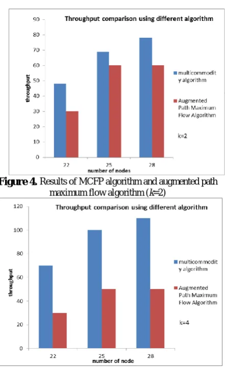
As the scale of small satellite network is not large, we define three scenarios of small satellites network to explore the influence of topologies and after extending TEG, there are respectively twenty-two, twenty-five and twenty-eight nodes in the graph. We assume that the capacities of all edges in the graph are twenty, except the infinity edges defined before and we set several source-sink demand pairs corresponding to specific demands. To investigate the effect of different algorithms, we choose a general method called augmented path maximum flow algorithm that is using single commodity max-flow algorithm for each source-sink demand pairs in sequence and augmenting the residual network graph every time after the single commodity max-flow is implemented. Then we will compare our MCFP algorithm with the augmented path maximum flow algorithm.

Figure 4.Results of MCFP algorithm and augmented path

maximum flow algorithm (k=2)

Figure 5. Results of MCFP algorithm and augmented path

maximum flow algorithm (k=4)

Results of the two algorithms are shown in the Fig.4 and Fig.5. The augmented path maximum flow algorithm is able to obtain the maximum throughput between single source-sink nodes, it cannot collaboratively optimize the maximum flow path traffic for multiple source-sink node pairs and the optimization of routing performance cannot

be achieved. With different node numbers and different source-sink node pair requests, the small satellite network throughput of our method based on TEG model is obviously larger than that obtained by using the augmented path maximum flow algorithm. Furthermore, comparing the results of two source-sink demand pairs and four source-sink demand pairs, the difference between the two algorithms is more obvious with four source-sink demands. We can see that the more complicated the topology is as well as the more demands it has, MCFP algorithm will have better effects than general solution.

Figure 6. Throughput v.s.  with 20 nodes (k=4)

Table 1.The change of 



Iteration

s

Time(s) throughp

ut

0.5 98 0.184 5.136

0.4 165 0.265 6.053

0.3 314 0.429 7.055

0.2 758 0.999 8.219

0.15 1395 1.672 8.861

0.1 3244 3.700 9.538

Both Fig.6 and Table.1 show the details for the algorithm to solve the TEG graph of a satellite network with 22 vertices and 36 edges.

To explore the dependency on



, we use the algorithm to solve a flow network of small satellite where the optimal throughout (OPT) is 9.9. OPT is marked as the gray horizontal line at the top in Fig.6 and the closer to

OPT



is, the better results we get. The figure also shows the (1 3 )  approximation guarantee of the solution. The guarantee says that the algorithm will produce a flow F

such that (1 3 )  OPT F OPT, where F is the size of the flow. This guarantee means that the algorithm will produce a flow that its throughput is extremely close to

OPT, in another word ,is above the guarantee line, and under the OPT line.

EAI Endorsed Transactions on

The values of



, iterations, running time and throughput can be found in Table.1. To look in detail, as the number of



decreases, the algorithm needs more iterations and time to get the solution and the final throughput will be more optimal. From another point of view, if the network changes fast and requires making decision quickly and in time, choosing a reasonable



to achieve the balance of the running time and the accuracy is a wise choice.

4. Conclusion

We apply the traditional time-expanded graph to model the data acquisition of small satellite network and use an approximation method to accelerate the solution for MCFP and make global optimization of routing between satellite network nodes. The quantitative comparison between our MCFP algorithm and general augmented path maximum flow algorithm proves the algorithm achieving better throughput and being closer to the optimal solution. Exploring the detail of the algorithm, we conclude that we need to make a reasonable selection of parameter in our algorithm for satellite network nodes communication to achieve the balance of the running time and the accuracy.

References

[1] R. S. Jakhu and J. N. Pelton, Small Satellites and Their Regulation. New York, NY, USA: Springer, 2014.

[2] L. R. Ford and D. R. Fulkerson, Flows in Networks.

Princeton, NJ, USA:Princeton Univ. Press, 1962.

[3] Runzi Liu, Student Member, IEEE, Min Sheng, Member,

IEEE, King-Shan Lui, Senior Member, IEEE, Xijun Wang, Member, IEEE, Yu Wang, and Di Zhou, “An Analytical

Framework for Resource-Limited Small Satellite

Networks,” IEEE COMMUNICATIONS LETTERS, vol. 20, no. 2, February. 2016.

[4] Shimon Even, Alon Itai, and Adi Shamir. On the

complexity of time table and multi-commodity flow problems. In Foundations of Computer Science, 1975., 16th Annual Symposium on, pages 184–193. IEEE, 1975.

[5] Masao Iri. On an extension of the maximum-flow

minimum-cut theorem to multicommodity flows. Journal of the Operations Research Society of Japan, 13(3):129– 135, 1971.

[6] Farhad Shahrokhi and David W Matula. The maximum

concurrent flow problem. Journal of the ACM (JACM), 37(2):318–334, 1990.

[7] Neal E Young. Randomized rounding without solving the linear program. In SODA, volume 95, pages 170–178, 1995.

[8] Naveen Garg and Jochen Koenemann. Faster and simpler

algorithms for multicommodity flow and other fractional packing problems. SIAM Journal on Computing, 37(2):630–652, 2007.

[9] Lisa K Fleischer. Approximating fractional

multicommodity flow independent of the number of

commodities. SIAM Journal on Discrete

Mathematics,13(4):505–520, 2000.