Modeling the Connections of Dynamic Sensor Fields
Based on BT-Graph
Tuyen
Phong
Truong
1,*,
Huong
Hoang
Luong
2,
Hiep
Xuan
Huynh
2,
Vinh
Cong
Phan
3and
Bernard
Pottier
11Lab-STICC, UMR CNRS 6285, Université de Bretagne Occidentale, France 2Can Tho University, Vietnam
3Nguyen Tat Thanh University, Vietnam
Abstract
In this article, we propose a new approach to model and optimize the dynamic sensor field for both internal network connections and LEO satellite connection based on BT-Graph. Due to the shift of LEO satellite’s orbit at each revolution, a dynamic sensor field (DSF), which is able to redetermine its gateways, is suitable to improve successful data communications. It is convenient to present a DSF as a BT-Graph that aims to utilize optimization algorithms. Parallel search algorithms are also deployed for more efficient execution time when DSFs consist of a significant large number of nodes. The simulation experiments are performed on an abstract forest fire surveillance network to validate our proposed approach.
Receivedon 02 January, 2016;acceptedon 10 February, 2016;publishedon 09 March, 2016 Keywords: associate analysis, BT-Graph, parallel processing, sensor field, LEO satellite.
Copyright© 2016 T. P. Truong etal.,licensedto EAI.This isanopen accessarticledistributedunderthetermsofthe Creative Commons Attribution license (http://creativecommons.org/licenses/by/3.0/), which permits unlimited use,distributionandreproductioninanymediumsolongastheoriginalworkisproperlycited.
doi:10.4108/eai.9-3-2016.151116
1. Introduction
Wireless Sensor Network (WSN) [1] is known as a network of sensors cooperatively operating in order to surveillance or collect the environmental parameters. Although the short transmission range can be compensated by applying a mesh topology, it would be economically infeasible to deploy in large geographic areas or behind obstacles (mountains, oceans, ...). To overcome these disadvantages, satellite-based wireless sensor networks have emerged as a promising technology with various applications.
Because the orbit of a LEO satellite shifts in westward direction around the polar axis at each revolution [12], the meeting points of a gateway on the Earth’s surface and the LEO satellite will be changed over time. With a static sensor field, it can be occasionally unsuccessful in communication with the LEO satellite because the meeting time is not enough for data exchange [12]. Therefore a dynamic sensor field (DSF) [1], which has the ability to redetermine its gateway to adapt with the
∗
Tuyen Phong Truong. Email: [email protected]
shifts of LEO satellite’s paths, is proposed to improve the connection time.
It is necessary to choose proper gateways for the longest length of connection time. Consequently, the connections between a LEO satellite and a dynamic sensor field should be presented by a graph-based model because it is convenient to determine number of neighbors in the satellite’s communication range and then apply the optimization algorithms. Moreover, BT-Grap model [2] based on balltree structure is efficiently support not only for searching the range nearest neighbors (RNN) but also finding the shortest path to a given target node [4] [18] [20]. In this article, we propose a new approach, namely dynamic sensor field optimization model based on BT-Graph (BT-DYNSEN), to model and optimize the DSF in communication with LEO satellite.
In addition, with the development of Compute Unified Device Architecture (CUDA), general purpose Graphics Processing Unit (GPGPU) is widely used to implement parallel algorithms, which can speed up the large and complex processing tasks [7] [8]. Nonetheless, serial graph algorithms are hard to be parallelized on GPUs due to irregular memory access and huge
on
C
ontext-aware Systems and Applications
memory-intensive operations. For this reason, we also propose parallel algorithms to improve search speed based on BT-Graph model using NVIDIA CUDA GPUs. In our work, the experimental results were deployed on parallelization of RNN algorithm and Dijkstra’s shortest path search algorithm.
The rest of this article is organized as follows. In section 2, we overview related works. Section 3 presents the graph-based model for a DSF based on BT-Graph (BT-DYNSEN). How to optimize the DSF for satellite connection is presented in section 4. Implementation of BT-DYNSEN is described in section 5. Section 6 gives the simulation experiments on an abstract network for forest fire surveillance in Vietnam before a conclusion is drawn.
2. Related work
The LEO satellite communication can be used in mobile satellite communications, surveillance the Earth surface, geological surveys, so on [1] [16] [19]. In the last decade, researches on communication services provided by LEO satellites have focused on several main directions such as optimizing the mechanics, interconnections, electric circuits, power supply. On another approach, many surveys show the research topics in design trajectory, handover traffic and constellation, as well as design protocols, radio frequencies, onboard transceivers and antenna designs [13] [14] [1] [19]. However, the direct radio links between sensor fields and LEO satellites are not considered in literature. In recent years, it emerges as an attractive topic because of the current innovation solutions such as LoRa Semtech and solutions from vendors QB50 [11].
Furthermore, graph-based model has emerged as well approach to present the structure and elaborate the performance of wireless sensor networks [3]. For example, random geometric graph [20] was used to determine the probability of the whole network being connected. Secure communications between large number of sensor nodes in WSNs can be elaborated on expander graph [25] and finding transmission path in network was performed based on Pascal graph [5]. Furthermore, hyper-graph [24] was utilized to support for reducing the transmission energy consumption and improving the fault-tolerant ability of the system.
Additionally, in recent years parallelization on GPU platforms is an emerging strategy to improve significantly performance speed [9]. When the graph consisting of a vast number of nodes, it is necessary to process in parallel based on NVIDIA CUDA technology to improve search speed [10]. In the next section, we introduce BT-DYNSEN model for optimizing the DSF for the connection with LEO satellite.
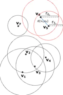
Figure 1. A dynamic sensor fiel in which the
communicationranges of sensor nodes are indicated by the radii of balls.
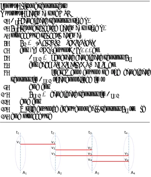
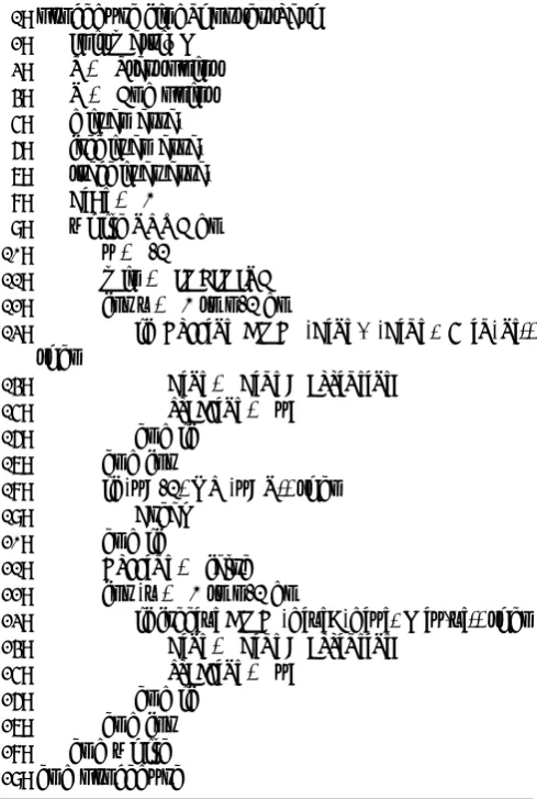
Figure 2. A BT-Graph of the dynamic sensor fiel with
07 vertices V ={v1, v2, v3, v4, v5, v6, v7} and 5 edges
E={e1=e(v1, v2), e2=e(v1, v3), e3=e(v2, v3), e4=
e(v3, v4), e5=e(v5, v6)}.
3. BT-DYNSEN
3.1. BT-DYNSEN modelof DSF
BT-DYNSEN model of a dynamic sensor field (DSF) [1] based on BT-Graph [2] is a graph G(V,E). In this graph, set of vertices V ={vi}, i= 1..n corresponds to
sensor nodes and set of edges, E={ej}, j= 1..m are
connections between the nodes with associated weight functions W ={wj}, j= 1..m. The value of each wj is
given by Euclidean distanced(vi, vj),i,j. Additionally,
R={ri}, i= 1..n are the radii of the communication
ranges of nodes [2] [4] [6]. An edge is established if and only if the distance between two nodes is less or equal to the minimum value of their communication radii, d(vi, vj)≤min(ri, rj), i,j. Note that the terms nodeandvertexare used interchangeably in this article as a matter of convenience.
In Figure1, for an example, a pair of vertices (v5, v6) has communication ranges r5 and r6 respectively. Because the distance betweenv5 andv6 is less thanr,
d(v5, v6)< r, so there exists an edgee5connecting them as can be seen in Figure 2. Similarly, the others edges
2
EAI
European Alliancefor Innovation
EAI Endorsed Transactions on Context-aware Systems and Applications
Table 1. Anexampleofsatellite connectiondata withthreerows: Connection number,Connection vector andTime vector.
Connectionnumber 1 2 3 ... Connectionvector v1 v3 v4 ...
Timevector t1 t2 t3 ...
of this graph namely e1=e(v1, v2), e2=e(v1, v3), e3=
e(v2, v3), e4=e(v3, v4) could be established. There are 2n−5 edges between a pair of nodes of this graph that
are not existed due to inadequacy of the condition. The vertexv7is isolated because all distance values between it and the other nodes are inadequate to the condition.
3.2. BT-DYNSEN modelof LEO satellite connection
The connections between a LEO satellite and a dynamic sensor field are also described in a BT-Graph. Let V ={vi}, i=1..n, is a set of sensor node coordinates in a DSF.
In this scenario, connection time is defined when any sensorset [1] of the DSF under the satellite coverage. The LEO satellite communication range is considered as a circle whose center is sub-point on the ground (sub-satellite point), s. It is noted that sub-satellite point,
s, is where on the ground the straight line connecting the center of the Earth and the satellite meets the Earth’s surface [12]. The associated BT-Graph consists ofn+ 1 verticesP ={V , s}={v1, v2, ..., vn, s}. If a node is
within the communication range of the satellite, there exists an edge with weight given by the Euclidean distance between them. Otherwise edge weight is set to infinity. Consequently, the number edges of the graph arem+nby addingnnew edgesC={c1, c2, ..., cn}with
ci =c(s, vi), i= 1..n. The weights of the n new edges are denoted by Z={z1, z2, ..., zn}. In this case the set
of edges isR={E, C}={e1, e2, ..., em, c1, c2, ..., cn}and the
set of corresponding weights isQ={W , Z}={{wk},{zi}}
with k= 1..m, i= 1..n. Hence the BT-DYNSEN model for LEO satellite connections is presented by a graph G(P,R) with weight functions Q.
Furthermore, during the connection time only one sensor node (vertex) of a dynamic sensor field is chosen to connect with the sub-satellite point (center vertex) at one time [1]. A number of different nodes could be chosen based on the value of edge weights at different times. To manage the connections, the name of chosen node is kept inConnection vector[1] and the corresponding time is saved in Time vector [1] (as in Table1).
Table 1 shows that in connection 1, center vertex
s connects with v1 at time t1. In a similar way, in connection 2 at time t2 and connection 3 at time t3,v4 andv2are chosen to connect withsrespectively.
For instance, Figure 3 shows three graphs of the dynamic sensor field in three different connections with the center vertex s (a sub-satellite point) at different
Figure 3. The BT-Graph of a dynamicsensor fiel in three
di˙erentconnections(solidred lines) at timest1, t2 andt3.
Figure 4. Gateway of sensorfiel geometry[12].
Figure 5. Relationshipbetween sensor node of a DSF and
sub-satellite point[12].
times t1, t2 and t3. At time t1 (Figure 3(a)), vertex
v1 is chosen and edge c1 is established. Similarly, in Figure3(b) and Figure3(c) vertexv3,v4 are chosen for connections that leads to corresponding edgesc3,c4are established at timet2andt3respectively.
3.3. Computethe connectiontime
In this section, we describe the way to calculate connection time, tij, between a LEO satellite and a gateway of DSF, vj [1] [12] [15]. Similarly, the calculation could be applied for all other nodes. Note that every node of the sensor field is assumed as a gateway for the connection with the satellite in calculating the values of connection time.
First, it is necessary to define the angles and related distances between satellite, a gateway on the ground and the Earth’s center. The parameters are indicated on Figure4. For angular radius of the spherical Earth,ρi, and the angular radiusλ0i can be found from relations
sin(ρi) =cos(λ0i) =
RE
RE+H
(1)
whereRE= 6378.14 km is the Earth’s radius andHis the altitude of the satellite above the Earth’s surface.
With the coordinates of a sub-satellite point, si (Longsi, Latsi) along each satellite’s ground track and a sensor node, nodes vj of the DSF (Longvj, Latvj), and defining∆Lij =|Longsi−Longvj|, the azimuth,ΦEij, measured eastward from north, and angular distance,
λij, from the sub-satellite point to the sensor node (see Figure5) are given by
cos(λij) =sin(Latsi)sin(Latvj)+
cos(Latsi)cos(Latvj)cos(∆Lij)
(3)
cos(ΦEij) =((sin(Latvi)−
cos(λij)sin(Latsi))/(sin(λij)cos(Latsi)) (4)
where ΦEij <180 deg if vi is east of si and ΦEij > 180 deg if vi is west ofsi. Consider triangleOsivj (in Figure 4), the distance, dij, between si and vj can be found using the law of cosines:
dij2 =R2E(1−cos(λij)) (5)
Theconnection time,tij, is given by
tij = (
P
180deg) arccos(
cos(λijmax) cos(λijmin)
) (6)
wherePis theorbit periodin minutes. From Equations (5) and (6), the communication duration, tij, strongly depends on how close the nodesvjis to the sub-satellite pointssi, the distancesdij, along the ground track on any given orbit pass [12].
3.4. Constraint
The altitude of a LEO satellite must be in range from 275 km to 1400 km due to atmosphere drag and Van Allen radiation effects [12]. Besides, the experimental results were announced by High Altitude Society in United Kingdom that LoRa SemTech transceivers can communicate in distance up to 600 km in environment without any obstacle and 20-40 km in urban area [22]. Based on these factors, maximum communication range for all nodes in long range sensor fields is 40 km in this work. LEO’s satellites are chosen in our experiments must have the orbit altitude less than 600 km. Furthermore, the satellite’s relative speed over a fixed point on the Earth’s surface must be around 7.5 -8.0 km/sec [12]. The speed of the satellite is calculated by
v=
r
GmE
RE+H
(7)
Equation 7 shows that the speed of the satellite in orbit is in inverse proportion of its altitude [12]. Where
G is universal gravitational constant (G= 6.67x10⁻¹¹ Nm2/kg2) and mE is the mass of the Earth (mE= 5.98x1024 kg). With orbit altitude of satellite in range 300-600 km, the speed of satellite on orbit must be in range 7.56-7.73 km/sec.
4. Optimization method
4.1. Verify the connectivityof DSF
In this work, top down construction algorithm is chosen in order to build balltree structure for verifying the network connectivity of the DSF. In this manner, the time complexity can be found inO(nlog2n) [6].
Algorithm 1Verify the network connectivity of a DSF
1: procedureverifyConnectivity(D)
2: ifD.hasAPoint()then
3: Create a leaf B is a point in D
4: Return B
5: else
6: Let c is the dimension of greatest spread 7: Let L, R are the set of points lying to 2 subsets 8: Let r is a radius of ball
9: Create B with two children:
10: B.center←c
11: B.radius←r
12: B.leftChild←balltreeConstruct(L)
13: B.rightChild←balltreeConstruct(R)
14: end if
15: end procedure
Top down algorithm to construct the balltree is a recursive process from top to down. The process at each step is to choose the split dimension it and then split the set of values into two subsets. First, it is necessary to choose the point in the ball which is farthest from its center,p1, and then choose a second point p2 that is farthest from p1. It is followed by assigning all points in the ball to closest one of two clusters corresponding top1andp2. Finally, the centroid of each cluster is calculated and the minimum cluster radius for enclosing all the points are determined. This process is stopped only when the leaf balls contain just two points. Note thatDdenotes current considered balltree structure and B denotes leaf node defined after each process.
4.2. Determinethe sensorsets correspondingto each
sub-satellite point
Defining a sensorset [1] based on BT-DYNSEN is to find
k nearest sensor nodes (neighbors) under the satellite’s coverage area at each sub-satellite. It is a depth-first traversal algorithm for traversing tree or graph data structures, starting with the root node. The value ofQ
4
EAI
European Alliancefor Innovation
EAI Endorsed Transactions on Context-aware Systems and Applications
is updated during search process. At each considered node B,Qobtainskpoints which are nearest queryqas following algorithm.
Algorithm 2Determine a sensorset
1: proceduredetermineSensorset
2: ifballtreeNode.isALeafthen
3: ifd<query.rangethen
4: Write name of balltreeNode to file
5: end if
6: else
7: ifd<(query.range + radiusNode)then
8: left←balltreeNode.leftChild
9: right←balltreeNode.rightChild
10: rnn: left, query 11: rnn: right, query
12: end if
13: end if
14: end procedure
There are two different cases in BT-DYNSEN algorithm as follows. If current considered node is a leaf node and the distance from query point q toB is less than r (d < r), the obtained result is updated by addingBintoQ. Otherwise, ifBis not a leaf node and the distance from query pointqtoBis less than the total ofrand the radius of B (d < r+B.radius), it is necessary to perform recursive algorithm for the two child nodes of a parent node B: left-child and right-child.
4.3. Select the gateways of DSF
If a DSF, V, has n nodes, there are 2n−1 connection
items,G={gl}, l=1..(2n−1). It is necessary to find out
a set of proper nodes which play as gateways of DSF to provide the longest length of time for the connection. To do this, theassociation analysis algorithm[18] is applied. In this way, a DSF is represented in a binary format, where each row corresponds to a connection item and each column corresponds to a node. A node value is one if the node appears in a connection item and zero otherwise. Weight of a connection item determines how often a connection item is applicable to a set of connection items. The weight of a connection item,gi ∈
G, can be defined asw(gi) =| {gl |gi ⊆gl, gl ∈G} |, where the symbol|.|denotes the number of elements in a set.
The algorithm for selecting the gateways of the DSF is briefly presented in following list.
For example, a DSF with 4 nodes,V ={v1, v2, v3, v4}
is shown in Figure6. There are 4 sensorsetsA1 ={v1},
A2={v1, v2, v3}, A3={v2, v3, v4} and A4={v3, v4}. The weights of connection items are presented in Table 2. The connection with the highest weight corresponds to the least number of times required to change the gateways. It leads to the connection duration time of the
Algorithm 3Select the gateways of a DSF
Input: list of sensorsets
Output: gateways of DSF
1: Ck: candidate sensors (size k) 2: Lk: set of selected gateways (size k)
3: procedureselectGateway
4: L1← {weight1−sensorsets}
5: for(k=2;Lk.count>0;k++)do
6: Ck+1←generate candidate sensorsLk
7: for eachtransaction t∈datado
8: Increment count of the candidate
sensors inCk+1that contained in t
9: end for
10: Lk+1←candidate sensors inCk+1
11: end for
12: Write counted frequent of all sensorsLkto file
13: end procedure
Figure 6. The connectionsbetweena 4-node DSF with a LEO
satellite.
Table 2. The weightsof connectionitemsin a DSF with4 nodes.
Connectionitems Weights (v1,v2,v4) 1 (v1,v2,v3) 1
(v1,v3) 3
(v1,v3,v4) 1
connection is longest. Because the weight of connection item (v1, v3) is highest, this connection is chosen.
4.4. Find shortest path for data dissemination
The problem of finding shortest path from each sensor node of DSF to the gateway can be solved by a graph search method. The algorithm is presented as Algorithm 4.The algorithm proceeds in three following steps. First, the balltree graph-based model,G, is constructed. At the next step, the weight matrix M for edges connect each pair of vertices (sensor nodes) in V is computed based on their coordinates. Forvi,vj are two different vertices inV, in case ofvi ≡vj the edge weight is 0. If
vi .vj, the edge weight is given byd(vj, vj) ifd(vj, vj)≤
r, otherwise it is infinity,∞. Finally, the shortest path
Algorithm 4Find shortest path from each sensor node of DSF to the gateway
1: procedurefindShortestPath
2: Init matrix M 3: S←Start point
4: T←End point
5: dis an array 6: freeis an array 7: traceis as array 8: d[S]←0
9: whileTRUEdo
10: u←-1
11: min←INFINITE
12: forv←0ton-1do
13: if f ree[v] AND (d[v]>(d[u] +M[u, v]))
then
14: d[v]←d[u] =arr[u][v];
15: trace[v]←u;
16: end if
17: end for
18: if(u=-1) OR (u=T))then
19: Break
20: end if
21: f ree[u]←false
22: for(v←0ton-1do
23: iffree[v] AND (d[v]>(d[u]+M[u,v]))then
24: d[v]←d[u] =arr[u][v];
25: trace[v]←u;
26: end if
27: end for
28: end while
29: end procedure
that q is starting point (a sensor node) and e is the destination point (the gateway of DSF).
4.5. Parallelizationof RNN algorithmto determine
sensorsets
As mentioned in section 4.2, range nearest neighbors (RNN) search method on BT-Graph can be used to determine the set of nodes in a sensorset associated with each position of satellite along ground track. In this section, a greedy algorithm is proposed to nearest neighbors search running on CUDA (namely RNN-CUDA as shown in Algorithm 5). The process of this greedy algorithm consists of two part. One part is parallel processes on GPU to compute distances from query the point to all nodes of a dynamic sensor field. Another part runs on CPU to sort the obtained distances in ascending order and then pick upkneighbor nodes associated with shortest distance values.
Algorithm 5RNN-CUDA
1: .Host program executed on CPU
2: Load data into global memory 3: Assign the value of k
4: Copy data from CPU→GPU
5: .Parallel programs executed on GPUs
6: Compute distances from query point, q, to all nodes
v∈V
7: Copy data back from GPU→CPU
8: .Host program executed on CPU
9: Sort the distance values as a ascending list
10: Pick up k nearest neighbor nodes associated to k first value of the list
11: Release GPU memory
Figure 7. The flo chart of parallel Dijkstra algorithm for
searchingBT-Graph model.
4.6. Parallelizationof search algorithmto fin the
shortest path for data dissemination
To parellelize Dijkstra algorithm, we propose that each edge of BT-Graph is handled by a thread of CUDA. Figure 7 depicts the flow chart of parallel Dijkstra algorithm for searching BT-Graph model in which two procedures,Extract minandUpdate cost, are performed on NVIDIA GPUs. The parallelization of Dijkstra’s algorithm is illustrated in Algorithm 6.
5. BT-DYNSEN implementation
We have developed the BT-DYNSEN tool in C/C++, that enables to model and optimize the connection time between a dynamic sensor field with a LEO satellite. GPredict [17] is used to provide the information about BEESAT-3 satellite’s path. Besides, NetGen tool [21] is utilized to generate the abstract network of a 50-node dynamic sensor field from geographic data provided by Google maps service. The obtained result are the nodes of the DSF which should be configured as gateways for the best connection duration time and the shortest paths for data dissemination from each node to these gateways.
6
EAI
European Alliancefor Innovation
EAI Endorsed Transactions on Context-aware Systems and Applications
Algorithm 6DijkstraCUDA
1: Step 1:
Initialize weight matrix (input vectors), start point and stop point
2: Step 2:
Allocate vectors in device memory corresponding to each edge of BT-Graph
3: Step 3:
Copy vectors from CPU (host) memory to GPU (device) memory
4: Step 4:
- Search for a free vertex u that has the least cost from the starting vertexStou
+ If no vertexu is found, either it exists a path or not
+ Otherwise, from u we continue to consider the other free vertices
- Use CUDA to specify the thread for searching the paths between the vertexuand the others
5: Step 5:
Copy results from GPUs memory to CPU memory 6: Step 6:
Free device memory and host memory
Figure 8. Verify dynamicsensornetworkconnectivity.(a) A
50-nodedynamicsensornetwork,(b) Balltree structureof the DSF, (c) Connectivityof the DSF.
6. Experiment
6.1. Experiment1: Verify networkconnectivity
The connectivity of the 50-node dynamic sensor network was verified by applying BT-DYNSEN as shown in Figre 8(a). Figure 8(b) depicts the balltree structure of this DSF in which there are 49 balls with radii from 10.124m to 321.165m. BT-Graph model then was utilized to ensure the full connectivity of all network nodes, the radius 30.497m was then chosen as shown in Figure8(c).6.2. Experiment2: Determinethe sensorsets
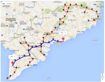
BT-DYNSEN tool was employed in determining sen-sorsets corresponding to sub-satellite points during vis-iting time. The map in Figure 9 shows the sensorset was determined with sub-satellites of BEESAT-3 at (lat-itude: 14.00, long(lat-itude: 102.48) in orbit 12794. Sub-satellite and Sub-satellite coverage were indicated by solid
Figure 9. Determinethe sensorsets correspondingto each
sub-satellite along the groundtrack of BEESAT-3 in orbit12794.
Figure 10. Select a set of nodeswhichplay as gateways of the
DSF accordingto the weightsof connections.
red square and red circle repectively. The sensorset consists of 19 sensor nodes which were under the satel-lite’s coverage area (the shadow area). There are four sensorsets were created along the BEESAT-3’s ground track in orbit 12794.
6.3. Experiment3: Select the gateways
With each sensorset, a subset of connections is established. The weights of each connection in subset are then computed. A set of connection items is created by combining these subsets. The best connection is chosen based on the weights of connection items. For instance, in Figure 10 node v36 was chosen as the gateway of the 50-node DSF to connection with BEESAT-3 satellite in orbit 12794 because its weight is highest in sensor nodes.
Figure 11. The shortest path for data disseminationfromnode
v50 to gateway nodev36.
Table 3. Comparisonon the executiontime of RNN BT-Graph
and RNN-CUDA.
N=10000, Q=10000 N=100000, Q=100000
RNN BT-Graph 179.46 17898.13
RNN-CUDA 123.47 5440.29
sensor nodes to the gateway. The interconnection weights within the DSF are geographic distances between each pair of nodes that were carried out by applying BT-DYNSEN model. Figure11, as an example, illustrates the chosen path (the bold blue line) for data dissemination from sensor nodev50to the gateway node
v36.
6.5. Experiment5: ParallelizationRNN algorithmfor
determiningsensorsets
In order to make the comparison between the parallel algorithms and serial ones for searching BT-Graph, we have run the simulations on a computer which is equipped with a INTELr Core i3-3220 3.3GHz processor, 4GB DDR3 SDRAM and a NVIDIA GeForce GTX660 graphic card. In our experiment, a comparison about BT-Graph’s search speed is obtained by performing both sequential algorithm on CPU and parallel algorithm on GPUs. On each algorithm with the same input data, which are generated randomly by program, experimental program is executed in 10 times for getting the average value of execution time.
The results is illustrated in Table 3, where N is the amount of initial data points andQis a number of query points. It shows that the search speed of RNN-CUDA be improved around 2.37 folds compared with that of RNN BT-Graph.
Figure 12. An executiontime comparisonof serial and parallel
Dijkstra’s algorithms.
6.6. Experiment6: ParallelizationDijkstra algorithm
for data dissemination
The purpose of this experiment is to compare search speed of traditional Dijkstra for BT-Graph and the corresponding speed of parallel Dijkstra (Dijkstra CUDA). The first step is to construct the weight matrix of BT-Graph model. Next, to obtain the average execution time, serial Dijkstra’s algorithm and parallel one are run in turns in 10 times. These experimental results are illustrated in Figure12.
From Figure 12, CPU can process efficiently for a small a number of vertices because it not waste extra time copying the data between CPU and GPU memories. Nevertheless, when a number of vertices are increased more than 8000, the duration time required for processing can be reduced significantly by using techniques of parallelism based on CUDA.
7. Conclusion
Based on BT-Graph, we have described a new approach in order to model and optimize the dynamic sensor field for LEO satellite connections. The distances between the sub-satellite points and each node of the sensor field is utilized as a key factor to find out the proper gateways for the longest connection time. The experimental results were obtained by applying several appreciate algorithms on BT-DYNSEN model to verify the connectivity of network, determine sensorsets at visiting time, choose set of gateway nodes and find shortest path for data dissemination in DSF. In order to improve the execution time, we implemented the corresponding parallel algorithms with CUDA on GPU, and analyzed its performance. The results show that the parallel algorithm on GPU is considerably superior to the serial one on CPU when BT-Graphs comprising more than 8000 vertices. Thus, our proposed graph-based model helps to increase the amount of time for data communications in long-range sensor field applications using satellite connections.
8
EAI
European Alliancefor Innovation
EAI Endorsed Transactions on Context-aware Systems and Applications
References
[1] Tuyen, P.T., Hoang, V.T., Hiep, X.H. and Pottier, B.
(2015) Optimizing the Connection Time for LEO Satellite Based on Dynamic Sensor Field. In 4th EAI International Conference on Context-Aware Systems and Applications
(ICCASA15), Vungtau, Vietnam.
[2] Huong, H.L.andHiep, X.H.(2014) Graph-based Model
for Geographic Coordinate Search Based on Balltree Structure. InProceeding of the17thInternational conference, Daklak, Vietnam, 116-123.
[3] Ines, K., Pascale, M., Anis, L. and Saoucene, M.
(2014) Survey of Deployment Algorithms in Wireless Sensor Networks: Coverage and Connectivity Issues and Challenges. In International Journal of Autonomous and
Adaptive Communications Systems (IJAACS), 24.
[4] Mohammad, R., Bijan, G. and Hassan, N. (2014)
A Survey on Nearest Neighbor Search Methods. In
International Journal of Computer Applications, 39-52. doi: 10.5120/16754-7073
[5] Panwar, D. and Neogi, S.G. (2013) Design of energy
efficient routing algorithm for wireless sensor network (WSN) using Pascal graph. InComputer Science & Infor-mation Technology, 175-189. doi: 10.5121/csit.2013.3217
[6] Omohundro, S.M. (1989) Five Balltree Construction
Algorithms. Technical Report.
[7] NVDIA, https://developer.nvidia.com/cuda-zone (accessed on 4 November 2015).
[8] GPU, http://www.nvidia.com/object/
what-is-gpu-computing.html(accessed on 4 November 2015).
[9] Gunjan, S., Amrita, T., Dhirendra, P.S. (2013) New
Approach for Graph Algorithms on GPU using CUDA. In
Internaltion Journal of Computer Application, Volume 72,
Issue 18, 38-42. doi: 10.5120/12645-9386
[10] Harish, P., Narayanan, P.J. (2007) Accelerating Large
Graph Algorithm on the GPU using CUDA. InProceeding
HiPC’07 Proceeding of the 14th international conference
on High performance computing, Vol. 4873, 197-208. doi:
10.1007/978-3-540-77220-0_21
[11] Lucas, P.Y., Long, N.H.V., Tuyen, P.T. and Pottier, B.
(2015) Wireless sensor networks and satellite simulation. In 7thEAI International Conference on Wireless and Satellite
Systems. doi: 10.1007/978-3-319-25479-1_14
[12] James, R.W.(2003) Space Mission Geometry. InWiley,
J.L. and textscJames, R.W. Space Mission Analysis and Design,3rdEdition(Microcosm Press), chap. 5.
[13] Cakaj, Sh., Keim, W.andMalaric, K.(2007)
Commu-nication Duration with Low Earth Orbiting Satellites. In
Proceedings of IEEE, IASTED, 4th International Conference
on Antennas, Radar and Wave Propagation, 85-88. doi:
10.1002/sat.4600090403
[14] Dosiere, F., Zein, T., Maral, G., Boutes, J.P. (1993)
A model for the handover traffic in low earth-orbiting (LEO) satellite networks for personal communications. In
International Journal of Satellite Communications, 574-578. doi: 10.1002/sat.4600110304
[15] Capderou, M. (2014) Ground track of a satellite. In
Capderou, M.[eds.]Handbook of satellite orbits from Kepler
to GPS(Springer International Publishing), chap. 8,
301-338. doi: 10.1007/978-3-319-03416-4
[16] Walter, C., Kris, S., Nicolas, D.andAdam, D.(2008)
Satellite based wireless sensor networks: global scale sensing with nano- and pico-satellites. In Proceedings of the6thACM conference on Embedded network sensor systems
(SenSys’08), 445-446. 10.1145/1460412.1460495
[17] Alexandru Csete, GPredict project,http://gpredict.
oz9aec.net/(accessed on 4 November 2015).
[18] Pang-Ning, T.,Michael, S.,Vipin, K.(2005) Association
Analysis: Basic Concepts and Algorithms. InIntroduction
to Data Mining (Addison-Wesley Longman Publishing
Co., Inc. Boston, MA, USA), chap. 6.
[19] Celandroni, N. et al. (2013) A survey of architectures
and scenarios in satellite-based wireless sensor networks:
system design aspects (International Journal of Satellite
Communications and Networking), vol. 31, 1-38. doi: 10.1002/sat.1019
[20] Dong, J., Chen, Q. and Niu, Z. (2007) Random
graph theory based connectivity analysis in wireless sensor networks with Rayleigh fading channels. In
Asia-Pacific Conference on Communications, 123-126. doi:
10.1109/APCC.2007.4433515
[21] Pottier, B.andLucas, P.Y. (2015) Dynamic
networks-NetGen. Technical report, Universite’ de Bretagne Occi-dentale, France.
[22] UK High Altitude Society, http://www. instructables.com/id/Introducing-LoRa-/step19/ LoRa-receiver-links/(accessed on 4 November 2015). [23] Berlin Experimental and Educational Satellite-2 and
-3. https://directory.eoportal.org/web/eoportal/ satellite-missions/b/beesat-2-3 (accessed on 4 November 2015).
[24] Ting, Y. and ChunJian, K. (2012) An energy-efficient
and fault-tolerant convergecast protocol in wireless sensor networks. In International Journal of Distributed Sensor Networks, 8 pages.
[25] Camtepe, S., Yener, B. and Yung, M. (2006)
Expander Graph based Key Distribution Mechanisms in Wireless Sensor Networks. In IEEE International
Conference on Communications, 2262-2267. doi:
![Figure 4. Gateway of sensorfiel geometry[12].](https://thumb-us.123doks.com/thumbv2/123dok_us/8412500.1691280/3.595.314.501.240.424/figure-gateway-of-sensorfiel-geometry.webp)