A Partial-differential Approximation for Spatial Stochastic Process Algebra

A Partial-differential Approximation for

Spatial Stochastic Process Algebra

Max Tschaikowski

Electronics and Computer Science

University of Southampton, UK

[email protected]

Mirco Tribastone

Electronics and Computer Science

University of Southampton, UK

[email protected]

ABSTRACT

We study a spatial framework for process algebra with or-dinary differential equation (ODE) semantics. We consider an explicit mobility model over a 2D lattice where processes may walk to neighbouring regions independently, and inter-act with each other when they are in same region. The ODE system size will grow linearly with the number of regions, hindering the analysis in practice. Assuming an unbiased random walk, we introduce an approximation in terms of a system of reaction-diffusion partial differential equations, of size independent of the lattice granularity. Numerical tests on a spatial version of the generalised Lotka-Volterra model show high accuracy and very competitive runtimes against ODE solutions for fine-grained lattices.

Keywords

Process Algebra, Fluid Approximation, Partial Differential Equations

1. INTRODUCTION

Modelling space explicitly is a relevant concern in a va-riety of disciplines such as biochemistry, ecology, and epi-demiology. At the same time, process algebra [13, 7, 8, 12, 2] have been successfully applied in the modelling of com-plex systems. Here we focus on spatial models expressed by process algebras with ordinary differential equation (ODE) semantics. We consider a spatial domain modelled as a regu-lar two-dimensional lattice, where agents may interact with each other if they are in the same region. In additions, agents may move independently from each other to neigh-bouring regions with an unbiased random walk, i.e., equally likely in any direction. The rate of movement, however, may be dependent on the agent type considered (and may be zero). Under these assumptions, the ODE state-space size grows linearly with the number of regions, making the analysis difficult in practice for dense lattices.

Our main contribution is a technique that, given a process algebra model, infers a system of partial-differential

equa-tions (PDEs) of reaction-diffusion type whose size is inde-pendent from the lattice size. This is an approximate view of the model which replaces discrete movements across regions in a continuous fashion. We work with the process algebra FEPA (Fluid Extended Process Algebra) presented in [19, 20]. However, with appropriate changes our ideas are appli-cable to languages such as Bio-PEPA [7], Cardelli’s Chemi-cal Ground Form [4], and the continuous_π-calculus [14].

In the literature concerned with models thatare not de-rived from a process algebra, such PDE approximations are typically presented by first considering astaticversion of the system in terms of an ODE model, where locality is not ex-plicitly taken into account. Such a static description defines the model of local interactions. Then, a spatial domain and a mobility model are added, leading to amobile model in terms of a PDE where a diffusive term captures movement, and a reactive term captures the interacting behaviour of the static model (cf., e.g., [16]). We proceed in an analo-gous fashion. The generic behaviour within any region is captured by some static FEPA model_M, where space is not modelled explicitly. Then, we consider a spatial lifting of the model, S(_M), a syntactic transformation which yields an FEPA model that makes the static version parametric with respect to the set of regions, and adds the random-walk behaviour. We justify our PDE approximation by observ-ing that the ODE system of the spatial modelS(_M) can be written in terms of a discrete Laplacian operator. The PDE is taken as the continuous approximation of such Laplacian. At first sight, this approximation might appear of little use in practice. This is because, except for special cases, analyt-ical PDE solutions are not available, and PDE systems are solved numerically using algorithms that discretise the con-tinuous space [18]. However, when solving the spatial ODE system directly the number of discrete regions is determined by the FEPA model, while the coarseness of the discrete mesh made by the PDE solver depends on the algorithm’s parameters. Thus, the PDE solver may in effect perform a coarsening of the original spatial domain. Numerical anal-ysis of spatial extensions of the generalised Lotka-Volterra model [15] confirm high accuracy for fine meshes.

Related work.

[3] studies mobile ad-hoc networks by means of a probabilistic process algebra. Potential fluid limits, however, are not investigated. PALOMA, instead, is a re-cently proposed stochastic process algebra with an explicit notion of space [9]. It assumes arbitrary spatial domain and mobility model, which can be captured by an ODE sys-tem but not as a PDE, as done here. MASSPA has an

3HUPLVVLRQWRPDNHGLJLWDORUKDUGFRSLHVRIDOORUSDUWRIWKLVZRUNIRU SHUVRQDORUFODVVURRPXVHLVJUDQWHGZLWKRXWIHHSURYLGHGWKDWFRSLHV DUHQRWPDGHRUGLVWULEXWHGIRUSURILWRUFRPPHUFLDODGYDQWDJHDQGWKDW FRSLHVEHDUWKLVQRWLFHDQGWKHIXOOFLWDWLRQRQWKHILUVWSDJH7RFRS\ RWKHUZLVHWRUHSXEOLVKWRSRVWRQVHUYHUVRUWRUHGLVWULEXWHWROLVWV UHTXLUHVSULRUVSHFLILFSHUPLVVLRQDQGRUDIHH

9$/8(722/6'HFHPEHU%UDWLVODYD6ORYDNLD &RS\ULJKWk,&67

'2,LFVWYDOXHWRROV

ODE semantics (also supporting higher-order moment clo-sures) with an explicit spatial domain, but with no move-ment [11]. Both PALOMA and MASSPA provide a process-algebra framework on top of the Markovian Agents Model [6]. Amobileextension of [6] is presented in [5], yielding a PDE. Space is directly continuous, instead of being interpreted as an approximation to a fine-grained lattice as done in this pa-per. The communication semantics is also different, being based on asynchronous exchange of messages, as opposed to a stricter notion synchronisation in FEPA. PALPS is a pro-cess algebra for spatial ecological modelling, proposed with a discrete-state semantics [17], allowing for individual-based reasoning which however does not scale to population mod-els. A review of other process algebras with explicit spatial support, but without PDE approximations, is given in [1]. Beyond process algebra, but closely related, is the spatial modelling technique for coloured Petri Nets in [10]. Tech-nically, we both assume a uniform lattice; conceptually, we both superimpose a spatial domain onto a static model. In-terestingly, their motivation is dual to ours: in [10] a contin-uous domain is discretised (allowing, e.g., to re-use Petri-net machinery), as opposed to our making discrete lattices con-tinuous.

Paper outline.

Section 2 overviews FEPA. Section 3 presents the spatial extension. Section 4 discusses the numerical eval-uation. Finally, Section 5 concludes.

2. FLUID EXTENDED PROCESS ALGEBRA

Next we present the fluid process algebra FEPA [20], here extended to allow birth and death of processes, needed in many models of biological and ecological systems. This is achieved made by considering a single-level grammar mixing sequential behaviour and parallel composition.

The notion offluid atomessentially defines the behaviour of an agent.

Definition 1. The syntax of a FEPA fluid atom is given by

S::=0_{|P |} i∈I

(_{αi, ri})_.S|SS

where _P def= _S denotes a constant, _α is an action in the

action setAand_r∈R>0.

As usual,0stands for the inert process. Choice between activities is encoded by_i∈I(_{αi, ri})_.Si. The value_riin ac-tivity (_αi, ri) denotes a coefficient that contributes to

deter-mining the rate of the exponential distribution at which the activity occurs. The parallel composition_SS is without synchronisation. Thus, an activity (_{α, r})_.(_SS) encodes a process that spawns two independent copies of_S. The se-mantics for a fluid atom is given by the following standard rules:

i∈I(αi, ri).Si

(αj,rj)

−−−−−→Sj

, j∈I S (α,r)

−−−→S P −−−→(α,r) S, P

def

=_S

S1−−−−→(α,r1) S1 S1S2−−−−→(α,r1) S1 S2

S2−−−−→(α,r2) S2 S1S2−−−−→(α,r2) S1S2 For a fluid atom_P, we denote the set of constants reachable from_PasB(_P). More formally,B(_P) is the smallest set such

that a)_P ∈ B(_P) and b) for any _P0 −−−→(α,r) _{P1 . . . Pn}

with_P0∈ B(_P), it holds that_{P1, . . . , P}n ∈ B(P), provided

that_Pi=0for all 1≤i≤n. Here, the equality is intended

to be syntactical.

We can now state the FEPA grammar for composing species.

Definition 2 (FEPA Model). A FEPA model_M is given by the grammar

M::=_MLM|P

where_L⊆ Aand_P is a constant. For any two distinct con-stants_P and_Pin_M, we require (without loss of generality) thatB(_P)∩ B(_P) =∅.

As usual,Lis the parallel operator; here synchronisation

takes place over shared action types belonging to the action set _L. For a FEPA model _M, we define G(_M) as the set of all constants in _M andB(_M) ={B(_P)|_P ∈ G(_M)}. Each fluid atom_P appearing in_M represents an indepen-dent population of agents of type_P. Thus, the model is com-pleted by aninitial concentration function _v(0) :_X→N0, with B(_M) ⊆ _X assigning initial conditions. A function v:_X→R_≥0is calledconcentration function.

Example 1. The well known SEIR (susceptible-exposed-infectious-recovered) model (e.g., [21]) can be described by the FEPA model_S{α}Iwith

Sdef= (_{α, r})_.0

Idef= (_α,1)_.(_IE) + (_{γ, z})_.R Edef= (_{β, s})_.I

where_α,_β and_γrefer to infection, exposure and recovery, respectively. We have thatG(_{S{α} I}) ={_{S, I}}, B(_S{α} I) =B(_S)∪ B(_I) ={_{S, E, I, R}}.

For conciseness, we present the semantics of interaction using only mass action. To encode PEPA [13], the version in [20] also allows minimum-based synchronisation which is however not used in the examples of interest here.

For an action _α, the apparent rate of a fluid atom _S is given by the sum of all rates labelled with_α that may be performed by _S. This allows to account for multiple _α -labelled choices such as_P def= (_{α, r})_.P+ (_{α, r})_.P.

Definition 3(Apparent Rate). The apparent rate of action

αof a fluid atom_S, denoted by_rα(S), is defined as follows:

rα(0) = 0,

rα(P) =rα(S) ifPdef=S

rα i∈I

(_{αi, ri})_.Si=

i∈I:αi=α

ri,

rα(S0S1) =rα(S0) +rα(S1).

Definition 4 (Parameterised Apparent Rate). Let_M be a FEPA model,_α ∈ Aand_v a concentration function. The apparent rate of_Mwith respect to_v is defined as

rα(M0LM1, v) =

rα(M0, v)·rα(M1, v) , α∈L,

rα(M0, v) +rα(M1, v) , α /∈L,

rα(P, v) =

Pi∈B(P)

vPirα(Pi)

where_rα(_Pi)is the apparent rate of a FEPA fluid atom_Pi, by Definition 3.

In Example 1 it holds that_rα(S, v) =rvS, which gives the

apparent rate at which a concentration of_vSS-components

exhibits action_α. When applied to a parallel composition, it gives the rate of interaction, e.g.,_rα(_{S{α}I, v}) =_rvSvI, which models the mass-action kinetics.

Parameterised component rates define the “fluxes” related to a species. These will be the constituents of the vector field of the ODE system to be analysed (shown below Definition 6). In the ODE for species _P, these will yield a negative contribution to_α-actions performed by_P, and positive for all contributions of other species_P.

Definition 5(Parameterised Component Rate). Let_Mbe a FEPA model,_α∈ Aand_va concentration function. The component rate of _P ∈ B(_M) is parameterised by_v in the following manner.

• M=_M0LM1: ifP ∈ B(Mi), i= 0,1, andα∈L

then

Rα(M0LM1, v, P) := Rα

(_{Mi, v, P}) rα(Mi, v) rα

(_{M0LM1, v})_.

• M=_M0L M1: ifP ∈ B(Mi), i= 0,1, andα /∈L

then

Rα(M0LM1, v, P) :=Rα(Mi, v, P).

• M=_Q: thenRα(Q, v, P) :=vPrα(P).

Notation.

We use Newton’s dot notation ˙_vP for the derivative of_vP. To enhance readability, time_twill be suppressed, e.g., ˙_vP denotes ˙_vP(t).

Definition 6. Let_M be a FEPA model. The fluid seman-tics of _M is given by_v˙ =_α∈AFα(M, v)≡F(M, v) with

initial condition_v(0)and_F(_{M, v})_P being defined as

α∈A P∈B(M)

pα(P, P)Rα(M, v, P)

− Rα(M, v, P),

where_P∈ B(_M)and

pα(P, P) :=

1 rα(P)

P−−−→(α,r) P₁...Pn

r· |{i|Pi=P}|

For instance,_S{α}Igives the well-known ODE system for the SEIR model:

˙

vS=−rvSvI v˙E=−svE+rvSvI (1)

˙

vI=−zvI+svE v˙R=zvI

Example 1 is non-spatial. More in general, as discussed, we take a FEPA model as a static description of the dynam-ics of interaction within any region of some spatial domain. In the remainder of this section we show how two further ex-amples from epidemiology and ecology of non-spatial models can be captured in FEPA. In the next section, instead, we consider the extension that can lift these models to a spatial domain. In passing, we note that none of the models pre-sented here can be encoded with the predecessors of FEPA [19, 20], because of the presence of birth/death behaviour.

Example 2(Predator/Prey Model). Let us define

Sidef=

1≤j≤d

(_αi,j, qi,jri,j).(SiSi) + (αi,j,(1−qi,j)ri,j).Si

+ (_βi, si).0

Rjdef=

1≤i≤d

(_αi,j,1)_.0+ (_{γj, zj})_.(_RjRj)_,

where0_{< qi,j<}1and1_{≤i, j≤d}. Then, the model

M:= (_{S1∅. . .∅Sd})_{αi,j|i,j}(_{R1∅. . .∅Rd}) (2)

induces the ODE system

˙ vSi=vSi

d

j=1

qi,jri,jvRj−sivSi (3)

˙

vRj =zjvRj−vRj

d

i=1 ri,jvSi

This is known as the generalised Lotka-Volterra model [15, Section 3.2], where the predators_{S1, . . . , Sd} prey on all the prey species _{R1, . . . , R}d, but with different severities ri,j.

With this agent-based view, _qi,j can be interpreted as the

probability that a predator _Si replicates after eating a prey

Rj.

Example 3(Competing Species). Let us define

S1def= (_{α, r1})_.(_S1S1S1)

S2def= (_{α, r2})_.(_S2S2)

Rdef= (_α,1)_.0

Then the FEPA process(_S1∅S2)_{α}Rinduces the ODE system

˙

vS1= 2r1vS1vR

˙

vS2=r2vS2vR

˙

vR=−(r1vS1+r2vS2)vR

Fluid atom_Rmodels a resource, which can be consumed with an_α interaction; _S1 is a species that gives rise to two de-scendants after consuming a resource, while_S2induces only one offspring. These ODEs are an instance of competitive Lotka-Volterra ODEs in the case of two species [15, Section 3.5].

3. SPATIAL FLUID EXTENDED PROCESS

ALGEBRA

In ecology, spatial models are explained as arising from their static counterparts by adding the Laplace operator

= _∂xx+∂yy [16, Chapter 10]. That is, if ˙v = f(v) is

a static ODE model its spatial version is given by apartial

differential equation_∂tω=_f(_ω) +_μω, with_μbeing the

diffusion coefficient. The usage of the Laplace operator is motivated by the fact that the spatial probability distribu-tion_π(_{t, x, y}) of a particle which is subject to a random walk satisfies the PDE_∂tπ=_π[15, Section 11.1].

In an analogous way, we take a FEPA process as the static model of the local interactions occurring within an arbitrary region, and define its spatial version in such a way that all fluid atoms are augmented with the capability of moving across neighbouring regions independently from each other,

in addition to enabling all the activities that are available in the static version. The transformation depends on the choice of the spatial domain, which we assume to be a discretisation of a square Ω ⊆ R2, denoted byR_K.1 The parameter_K determines the size of the region, i.e., we have thatRK :=

Ω∩(_K1Z)×(_K1Z), where_K≥1. Thus, the total number of regions isO(_K2).

The transformation from a static to a spatial model is carried out so as to have that processes never change region as a result of performing an activity originally present in the static version. For any static FEPA process_M, such a transformation is denoted bySK(M). In the present section

we show that the ODE system ofSK(M) is an

approxima-tion to the PDE system_∂tωP =_F(_{M, ω}) +_μPωP, with P ∈ B(_M).

We illustrate our intent behind the definition ofSK by

considering the predator-prey FEPA model (2) in the case of a single class of predators and preys (i.e.,_d= 1). To improve readability, we drop the superfluous index, i.e. _S ≡ _S1, α ≡ α1,1 and so on. Let us write N(x, y) for the set of (Neumann) neighbours of the region (_{x, y}), that isN(_{x, y}) is given by

RK∩ {(x−1/K, y),(x+ 1/K, y),(x, y−1/K),(x, y+ 1/K)}

Our transformation will yieldS_K(M) defined as

SK(M) =S(0,0)LR(0,0), L={αl|l∈ RK},

with

Sldef= (_αl_{, qr})_.(_Sl_Sl) + (_αl_,(1−_q)_r)_.Sl

+ (_βl_{, s})_.0+

l∈N(l)

(_{δ, μ}l,_Sl(_K))_.Sl

Rldef= (_αl_,1)_.0 + (_γl_{, z})_.(_Rl_Rl) +

l∈N(l)

(_{δ, μ}l,_Rl(_K))_.Rl_,

for all_l∈ R_K. Intuitively,S_K(M) models a situation where fluid atoms of typeB(_M) ={_{S, R}}move acrossR_Kvia the diffusion action_δ(which we assume in the remainder that it does not belong toA).

Such a transformation induces in effect a family of spatial

models depending on the choice of the rates_μl,_Pl(_K), which have not yet been defined. These may depend, in general, on the fluid atom_P that is moving, on the origin and target region, i.e.,_land_l, respectively, and on_K. The actions orig-inally available inM, i.e.,_α,_βand_γ, are instead performed locally, with the same rates as in the static model version

M. Enforcing synchronisation only between processes in the same region is achieved by appending_lto each action type, modifying the synchronisation sets accordingly in the model equation.

Hence, our idea of spatial extension is formally captured by the following.

Definition 7 (Spatial FEPA). For a given FEPA model

M, the spatial version of_M overRK, denoted bySK(M),

is inductively given by

SK(P) :=P(0,0)

SK(M0LM1) :=SK(M0)SK(L)SK(M1),

1_{This assumption simplifies presentation and} implementa-tion, but it can be in principle relaxed to arbitrary domains with a piecewise differentiable boundary.

whereSK(L) ={αl|α∈L∧l∈ RK}and, for alll∈ RK,

Pldef=

l∈N(l)

(_{δ, μ}l,_Pl(_K))_.Pl+ (α,r,i)∈X

(_αl_{, r})_.(_Pi,l_{1. . .Pi,n}l _i)

whenever _P def= _(α,r,i)∈X(_{α, r})_.(_{Pi,1 . . . Pi,ni}), where the case_μl,_Pl(_K) = 0corresponds to removing of the respec-tive summand in the definition of _Pl_{. (In the special case}

(_{Pi,1 . . . Pi,ni}) =0, we set(_Pl

i,1 . . . Pi,nl i) := 0.)

Moreover, letA+:={_αl_{|α∈ A ∧l∈ R}

K} ∪ {δ}.

For any FEPA model_M,SK(M) is a FEPA model, with

actions from A+. For any choice of the rates _μl,_Pl(_K), an underlying ODE system can be defined. For example, the ODE of_vSl inSK(M) is given by

˙

vSl=qrvSlvRl−svSl+

l∈N(l)

μl,lS(K)vSl−μ l,l S(K)vSl

,

where_l∈ RKandμl,lS(K)≥0. SinceRinduces|RK|ODEs

as well, the overall size of the system is 2_|RK|. In general, such a derivation is formally obtained through the following.

Theorem 1. Let us fix a FEPA model_M, a concentration function _v of SK(M) and some l ∈ RK. Then, the

con-centration function_v|l of_M, given by(_v|l)P :=vPl for all

P ∈ B(_M), satisfies the ODE_v˙_Pl =F(SK(M), v)Pl with

F(SK(M), v)Pl=F(M, v|l)P

+

l∈N(l)

μl,lP(K)vPl−μ l,l P(K)vPl

, P ∈ B(_M)_.

Proof. See Appendix A.

Informally, this theorem says that each ODE inSK(M)

has two contributions. The first contribution is thereactive

part_F(_{M, v|l})_P, which corresponds to the behaviour of the static model_M, accounting for local interactions within a region. Thediffusivepart, instead, is due to the migration across regions. A direct consequence of the above theorem is that the ODE system of a FEPA model_M overR_K has

|B(_M)| · |RK|coupled ODEs.

Now, we wish to study the conditions under which the analysis of_SK(_M) is independent from_K. Intuitively, we would like to make spacecontinuousby sending_Kto infin-ity, hence by making theRKincreasingly finer. This entails

turning per-region ODEs into a system of PDEs. For this, specific assumptions must be made on the choice of the rates

μl,Pl(K). In particular, a suitable scaling needs to be found

also with respect to_K. Further, we need to make assump-tions on the initial concentration function forS_K(_M) and how it scales with_K.

Overall, we make three assumptions, which we discuss in detail next.

Assumption 1: Unbiased Random Walk

.

We assume that each fluid atom is subjected to an unbi-ased random walk, i.e., it may migrate equally likely to any of its neighbours. More formally, we require that

(A1) _μl,_Pl(_K) =_μP(_K)

for all _P ∈ B(_M), _l ∈ RK and l ∈ N(l). Notice,

how-ever, that our assumption still allows distinct fluid atoms to perform migrations with different rates.

Assumption 2: Scaling of_μP(K)

.

Since a migration activity covers the distance 1_/KinRK,

each_μP(K) should scale withK in a reasonable way. To

motivate our forthcoming spatial scaling, let us consider an unbiased random walk in the two-dimensional unbounded grid _K1Z×_K1Z, where each migration covers the distance 1_/Kand the sojourn time at each state is exponentially dis-tributed with mean 1_/rK. Then, the corresponding CTMC, denoted by (_WK(_t))_t≥0, enjoys the following property. Proposition 1. Let us assume that_WK(0) = (0_,0)and de-note by_dK(_t) :=_WK(_t)the Euclidean distance of_WK(_t)

from the origin after time_t. Then, it holds that

E(_dK(_t)2) =rK K2

t, for all _K≥1 and _t≥0_,

whereE(·)denotes the expectation value.

Proof. See Appendix A.

Notice that if_rK = _K2_r1 for all_K ≥ 1, Proposition 1 yields

E(_dK(t)2) =E(d1(t)2), for all K≥1 and t≥0.

The above relation states that if each migration of the pro-cess covers a distance of 1_/K, then the migration rate should be_K2_r1, in order for the random walk to always coverthe same distanceon average independently of_K.

Thus, we define the scaling of the migration rates as

(A2) _μP(K) =μPK2, for all P ∈ B(M),

where_μP denotes some given nonnegative constant. When it is equal to zero, then_P-processes never move.

Assumption 3: Initial and Boundary Conditions

.

Whilst in the ODE interpretation (5) of spatial FEPA no particular restriction on the initial concentration function is needed, the PDE approximation can only make sense if v(0) converges, as a family of functions dependent on _K, to adifferentiable function on Ω as_K→ ∞. Thus, we fix partially continuously differentiable functions_ω0_P : Ω→R, where_P ∈ B(_M), and define the initial concentration as

(A3) _v(0)_P(x,y):=ωP0(x, y)

for_P∈ B(_M) and (_{x, y})∈ RK. This assumption establishes

the link between the PDE and the ODE interpretation. The initial condition_ωP0 evaluated at (_{x, y}) provides the initial concentration function for the ODE of the fluid atom_P(x,y). Finally, PDEs also require boundary conditions. In our model, the spatial domain isreflective, i.e., processes are not allowed to migrate outside the boundary. Formally, this cor-responds to setting Neumann boundary conditions (NBCs):

0 =_{∂xωP, ∂yωP}(_{x, y})_·ν(_{x, y})_, (4)

for all (_{x, y})∈_∂Ω and_t≥0, where_P ∈ B(_M) and_ν(_{x, y}) is the exterior normal vector at (_{x, y}) to the boundary_∂Ω of the square Ω.

Here, we wish to point out that by applying a minor change to the definition ofS_K(_M),absorbingboundary con-ditions could be encoded as well. While NBCs can be used

to model geographical barriers (e.g., an island), absorbing boundaries may be used to capture hostile environments (e.g., [16, Section 10.1]).

Definition 8 (Partial-differential Approximation). Let us fix a FEPA model_M and suppose that assumptions_(A1)– (A3) are satisfied forS_K(_M). Then, the underlying PDE system ofSK(M)is given by

∂tωP =F(M, ω)P+μPωP, P ∈ B(M).

The initial conditions are given by the functions_ωP0 : Ω→ R≥0, whereas the boundary conditions satisfy the NBCs (4). This is well-known in the literature as areaction-diffusion

PDE system (e.g., [15]), to highlight the role of the two summands in the time-derivative of _ωP, i.e., the reactive

part due to the local interactions and the diffusive part due to process migrations. Importantly, this PDE system has a size which is equal to|B(_M)|, the number of local states in the model’s static version_M.

We intend this PDE system as an approximation. Roughly speaking, the relation _v(0)_P(x,y) = ω0P(x, y) in(A3)

sug-gests that the ODE and PDE solutions satisfy_vP(x,y)(t)≈

ωP(x, y, t).

The nature of this approximation can be understood by considering the continuous Laplace operator appearing in the PDE system as the limit of thediscreteLaplace operator in the unit square. This is obtained by using Theorem 1 and assumptions(A1)and(A2). The spatial ODE system can be rewritten as:

˙

vPl =F(M, v|l)P+μP

(_K) K2

l∈N(l)

v_Pl−vPl

(1_/K)2

=_F(_{M, v|l})_P+_μPd_vPl, (5) where_P ∈ B(_M),_l∈ R_Kandd_v

Pl:=

l∈N(l)

_v

Pl−vP l (1/K)2

denotes the discrete Laplace operator for all inner regions l∈ RK. For instance, applied to Example 2, Equation (5)

reads

˙

vSl =qrvSlvIl−svSl+μSdvSl,

˙

vRl =zvRl−rvSlvIl+μRdvRl,

for all_l ∈ RK. Then, assuming that for sufficiently large

Kthe discrete Laplace operator can be approximated by its continuous analogue, we get the PDE

∂tωS=qrωSωI−sωS+μSωS,

∂tωR=zωR−rωSωI+μRωR,

where_ωP : Ω×[0;∞)→R_≥0. This is consistent with the PDE model that is already available in the literature (cf. [16, Chapter 10]).

As discussed, the PDE is used to provide an approximate estimate of the ODE solution of a modelS_K(_M), in a way that is however independent from_K(in the above example, using two PDEs only). In the following section we perform a numerical evaluation to assess the quality of this approxi-mation.

4. NUMERICAL EXAMPLES

For our tests we considered the predator-prey model of Ex-ample 2. We parameterised it for different number of species,

d= 1 _d= 3 _d= 5

K μ1 Time _μ2 Time _μ1 Time _μ2 Time _μ1 Time _μ2 Time

4 0.082 0 s 0.057 0 s 0.086 0 s 0.060 0 s 0.090 0 s 0.064 1 s 8 0.026 0 s 0.017 0 s 0.030 3 s 0.019 3 s 0.034 11 s 0.023 12 s 16 0.014 5 s 0.008 6 s 0.018 68 s 0.015 71 s 0.021 241 s 0.015 264 s 20 0.013 13 s 0.007 14 s 0.017 195 s 0.011 211 s 0.020 764 s 0.014 837 s

PDE Time 0 s 0 s 1 s 1 s 2 s 2 s

Table 1: Maximum absolute error between the ODE and PDE estimates of species_S1 at time0_.2 across the discrete mesh, for diffusion coefficients_μ1= 0_.10and_μ2= 0_.15.

−1 −0.5 0 0.5 1 0 0.1 0.2 0.3 0.4 0.5

(a) ODE Solution

−1 −0.5 0 0.5 1

0 0.1 0.2 0.3 0.4 0.5

(b) PDE Solution

Figure 1: _S1surfaces projected on the x-axis;_K= 20, d= 5, _μ= 0_.15.

d= 1_,3_,5, in order to study the impact on the PDE system size (equal to 2_d) of the static version of the model. We set the unit square Ω = [−1; 1]2as the spatial domain. We (arbi-trarily) fixed the parameters_ri,·=_i/20,_si=zi= (i+1)/20,

qi,j= 1. Instead, we experimented with two different

diffu-sion coefficients by setting_μSi=_μRi=_μ∈ {0_.10_,0_.15}for all 1≤_i≤_dto show the impact of mobility on the model’s dynamics. For each parameterisation of the model, we con-sidered spatial transformations with_K = 4_,8_,16, and 20, corresponding to increasingly finer discrete meshes with 92, 172, 332, and 412 regions, respectively. Thus each spatial transformation had migration rates equal to_μK2. In this way, all ODE systems with different values of_K(and other-wise same parameters) have the same PDE approximation.

The corresponding PDE system is, for all 1≤_{i, j}≤_d:

∂tωSi=ωSi

d

j=1

qi,jri,jωRj−siωSi+μSiωSi

∂tωRj =zjωRj−ωRj

d

i=1

ri,jωSi+μRjωRj

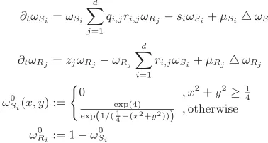
ωS0i(x, y) :=

0 _{, x}2+_y2≥1₄ exp(4)

exp(1/(1

4−(x2+y2))) ,

otherwise

ωR0i:= 1−ω0Si

The initial conditions,_ωS0_iand_ω0_Ri(bells centered at (0_,0) with peak 1_.0), are consistent with the NBCs.

As a measure of the accuracy, we considered solutions for species_S1 at time_t= 0_.20. These were chosen arbitrarily, the latter ensuring that the solution was sufficiently away from the initial condition. For each _K, the error is de-fined as the maximum absolute difference across the whole spatial domain between the ODE solution at each point in the discrete mesh and the corresponding PDE solution

(us-ing linear interpolation to sample at the same coordinate). Matlab R2013b was used for the numerical solutions. The ODEs were solved using the built-in_ode15sfunction, while the PDEs were solved using the function_parabolic in the Partial Differential Equation Toolbox. All parameters were set as the default ones. Runtimes were taken on a machine with 16 GB RAM.

Table 1 presents the results, showing high quality of the approximation in general. Figure 1, instead, visualises the numerical solutions of_S1. The range of values attained by the ODE/PDE solutions were within [0_.00; 0_.40], thus the absolute differences correspond to at most around 20% (for K= 4) relative to the peak values. The table shows higher accuracy with increasing_Kacross all tests (cf. Figure 1 for a visual appreciation). However, PDEs are cheaper to solve than ODEs for fine meshes. In fact, the ODEs could not be solved for significantly larger values of_Kdue to out-of-memory errors.

5. CONCLUSION

In this paper we considered a spatial extension of stochas-tic process algebra with ODE semanstochas-tics. Under the assump-tion of processes evolving over a two-dimensional regular lat-tice with an unbiased random walk, we have provided an ap-proximating reaction-diffusion PDE system. In our numer-ical tests, the quality of this approximation has been found to be highly accurate in the case of fine-grained lattices, at a much smaller computational cost. Pragmatically, tool im-plementation is ongoing. Theoretically, although here we focussed on ODE semantics only, future work will aim at in-vestigating convergence of the stochastic process underlying the process algebra to a PDE limit.

Acknowledgement.

This work was supported by the EU project QUANTICOL, 600708.

6. REFERENCES

[1] Bittig, A., Uhrmacher, A.: Spatial modeling in cell biology at multiple levels. In: Winter Simulation Conference. pp. 608–619 (2010)

[2] Buchholz, P.: Markovian Process Algebra: Composition and Equivalence. In: Proc. 2nd Workshop on Process Algebra and Performance Modelling. Erlangen, Germany (1994)

[3] Bugliesi, M., Gallina, L., Hamadou, S., Marin, A., Rossi, S.: Behavioural equivalences and interference metrics for mobile ad-hoc networks. Perform. Eval. 73, 41–72 (2014)

[4] Cardelli, L.: On process rate semantics. Theor. Comput. Sci. 391, 190–215 (2008)

[5] Cerotti, D., Gribaudo, M., Bobbio, A.: Presenting Dynamic Markovian Agents with a road tunnel application. In: MASCOTS. pp. 1–4 (2009)

[6] Cerotti, D., Gribaudo, M., Bobbio, A., Calafate, C.T., Manzoni, P.: A Markovian Agent Model for fire propagation in outdoor environments. In: EPEW, LNCS, vol. 6342, pp. 131–146. Springer (2010) [7] Ciocchetta, F., Hillston, J.: Bio-PEPA: A framework

for the modelling and analysis of biological systems. Theor. Comput. Sci. 410(33–34), 3065–3084 (2009) [8] De Nicola, R., Ferrari, G., Pugliese, R.: KLAIM: a kernel language for agents interaction and mobility. IEEE Trans. Software Eng. 24(5), 315–330 (1998) [9] Feng, C., Hillston, J.: PALOMA: A Process Algebra

for Located Markovian Agents. In: QEST (2014), to appear

[10] Gilbert, D., Heiner, M., Liu, F., Saunders, N.: Colouring Space — A Coloured Framework for Spatial Modelling in Systems Biology. In: Petri Nets, LNCS, vol. 7927, pp. 230–249. Springer (2013)

[11] Guenther, M.C., Bradley, J.T.: Higher moment analysis of a spatial stochastic process algebra. In: EPEW, LNCS, vol. 6977, pp. 87–101. Springer (2011) [12] Hermanns, H., Rettelbach, M.: Syntax, semantics,

equivalences, and axioms for MTIPP. In: Proceedings of Process Algebra and Probabilistic Methods. pp. 71–87. Erlangen (1994)

[13] Hillston, J.: A compositional approach to performance modelling. Cambridge University Press, New York, NY, USA (1996)

[14] Kwiatkowski, M., Stark, I.: The continuous pi-calculus: A process algebra for biochemical modelling. In: CMSB. pp. 103–122. No. 5307 in LNCS (2008)

[15] Murray, J.D.: Mathematical Biology I: An Introduction. Springer, 3rd edn. (2002)

[16] Okubo, A., Levin, S.A.: Diffusion and Ecological Problems : Modern Perspectives. Interdisciplinary Applied Mathematics, Springer (2001)

[17] Philippou, A., Toro, M., Antonaki, M.: Simulation and verification in a process calculus for

spatially-explicit ecological models. Scientific Annals of Computer Science 23(1), 119–167 (2013)

[18] Thomas, J.W.: Numerical Partial Differential Equations: Finite Difference Methods. Springer-Verlag (1995)

[19] Tschaikowski, M., Tribastone, M.: Exact fluid lumpability for Markovian process algebra. In: CONCUR. LNCS, vol. 7545, pp. 380–394 (2012) [20] Tschaikowski, M., Tribastone, M.: Extended extended

differential aggregations in process algebra for performance and biology. In: QAPL (2014), to appear. [21] Watson, R.K.: On an epidemic in a stratified

population. Journal of Applied Probability 9(3), pp. 659–666 (1972)

APPENDIX

A. PROOFS

A.1 Proof of Proposition 1

Although the the continuous-time random walk is well studied, we could not find a reference that shows Proposition 1.

Proposition 1. We give a proof which relies on the uniformi-sation method for CTMCs with countable state spaces2. Let (_WK(_n))_n≥0 denote the unbiased random walk in discrete

time on_K1Z×_K1Zwith_WK(0) = (0,0) and let (N(t))t≥0be the homogenous Poisson process with intensity_rK. Further, let_P denote the transition matrix of (_WK(n))n≥0. Then it holds that_WK(_t) =_WK(_N(_t)) and

E(_d2_K(_t)) = (x,y)∈Z2

PWK(t) =

_x

K, y K

_x

K

2 +

_y

K

2

=

(x,y)∈Z2

∞

n=0 e₍T0

K,K0)P

n(rKt)n

n! e

−rKt

e(x K,Ky)

_x2_+y2 K2

=_e−rKt

∞

n=0 (_rKt)n

n!

(x,y)∈Z2

e₍T0

K,K0)P

n

e(x K,Ky)

_x2_+y2 K2

= 1 K2e

−rKt

∞

n=0 (_rKt)n

n! E

WK(n)2

= 1 K2e−rKt

∞

n=0 (_rKt)n

n! n

= 1 K2e

−rKt

rKt

∞

n=1

(_rKt)n−1

(_n−1)!

=

_r

K

K2

t

A.2 Proof of Theorem 1

Lemma 1. Let us fix a FEPA model_M. Then it holds that

rαl(SK(M), v) =rα(M, v|l)

Rαl(SK(M), v, Pl) =Rα(M, v|l, P)

for all_P ∈ B(_M), _α∈ A,_l∈ R_K and concentration func-tions_v ofSK(M).

Proof. We prove this by induction on_M.

• M=_P0: The claim follows with

rαl

SK(P0), v

=

Pi∈B(P0)

rα(Pi)vP_il=rα(P0, v|l),

Rαl

SK(P0), v, Pl

=_rα(_P)_vPl =Rα(P0, v|l, P).

• M=_M0LM1: We assume without loss of generality

that_P ∈ B(_M0), which yields also_Pl _{∈ B(S} K(M0)).

Let us first consider the case_α ∈_L. Then, together with_αl_{∈ S}

K(L), we infer

rαl(SK(M0LM1), v) =rαl(SK(M0), v)·rαl(SK(M1), v)

I.H.₌

rα(M0, v|l)·rα(M1, v|l)

=_rα(M0LM1, v|l)

2_{See Section 2.1 of Chapter 8 in Br´emaud, P.: Markov} chains, Gibbs fields, Monte Carlo simulation, and queues. Springer-Verlag (1999)

and

Rαl

SK(M0LM1), v, Pl

=Rαl

SK(M0), v, Pl

rαl(SK(M0), v) rα

lSK(M0LM1), v

I.H.₌ Rα(M0, v|l, P)

rα(M0, v|l) r

α(M0LM1, v|l)

=Rα(M0LM1, v|l, P).

If_{α /}∈_L, it holds that_αl_{∈ S/}

K(L), yielding

rαl(SK(M0LM1), v)

=_rαl(SK(M0), v) +rαl(SK(M1), v)

I.H.₌

rα(M0, v|l) +rα(M1, v|l)

=_rα(M0LM1, v|l)

and

Rαl

SK(M0LM1), v, Pl

=_RαlSK(M0), v, Pl

I.H._{= R}

α(M0, v|l, P)

=Rα(M0LM1, v|l, P)

Theorem 1. Let us fix the unique √_P ∈ G(_M) such that P ∈ B(√_P). The claim follows then

F(S_K(_M)_{, v})_Pl =

=

α∈A+

P∈B(SK(M))

pα(P, Pl)Rα(SK(M), v, P)

− Rα(SK(M), v, Pl)

=

α∈A P˜∈B(√P)

pαl( ˜Pl, Pl)Rαl(SK(M), v,P˜l)

− Rαl(SK(M), v, Pl)

− Rδ(SK(M), v, Pl)

+

l∈N(l) pδ(P

l

, Pl)R_δ(S_K(_M)_{, v, P}l)

L1₌

α∈A P˜∈B(√P)

pα( ˜P , P)Rα(M, v|l,P˜)− Rα(M, v|l, P)

+

_l∈N(l)

μl,lP(K)vPl−μ l,l P(K)vPl

=_F(_{M, v|l})_P+

l∈N(l)

μl,lP(K)vPl−μ l,l P(K)vPl

.