Modelling and Simulating Systems Security Policy

Modelling and Simulating Systems Security Policy

Tristan Caulfield

[email protected]

David Pym

[email protected]

ABSTRACT

Security managers face the challenge of designing security poli-cies that deliver the objectives required by their organizations. We explain how a rigorous modelling framework and methodology— grounded in semantically justified mathematical systems modelling, the economics of decision-making, and simulation—can be used to explore the operational consequences of their design choices and help security managers to make better decisions. The methodol-ogy is based on constructing executable system models that illus-trate the effects of different policy choices. Models are compo-sitional, allowing complex systems to be expressed as combina-tions of smaller, complete models. They capture the logical and physical structure of systems, the choices and behaviour of agents within the system, and the security managers’ preferences about outcomes. Utility theory is used to describe the extent to which se-curity managers’ policies deliver their sese-curity objectives. Models are parametrized based on data obtained from observations of real-world systems that correspond closely to the examples described.

Categories and Subject Descriptors

I.6 [Simulation and modelling]: General; F.3 [Logics and mean-ings of programs]: Miscellaneous; H.1 [Models and principles]: Systems and information theory; K.6 [Security and Protection]; K.6.0 [General]: Economics; K.6.1 [Project and People Man-agement]: Systems analysis and design

General Terms

design, economics, experimentation, languages, management, mod-elling, security, theory

Keywords

composition, decision, location, logic, modelling, policy, process, resource, security, semantics, simulation

1. INTRODUCTION

A system’s security policies—and, indeed, a system’s management policies more generally—must be formulated so as to deliver the

declarative objectives of the system’s managers in the context of the system’s architecture and operational objectives.

When formulating, implementing, and monitoring security poli-cies, managers are often faced with deciding between achieving varying degrees of security and achieving varying degrees of oper-ational effectiveness. That is, more effective security controls will often more severely impede operations. A key challenge for system managers is to engineer trade-offs between concerns such as these that is acceptable to their organizations.

It is an increasingly commonplace observation that mathematical modelling—of the system, of its operational and security policies, and of the behaviour of its users—can provide useful decision-support tools [2, 3, 4, 5]. But the systems about which these de-cisions must be made are usually complex socio-technical systems of systems for which analytic solutions to policy-system co-design problems are rarely available. Instead, simulation-based models [18] supporting experimental mathematical modelling methods of-fer a useful approach [2, 4, 8, 5].

In this paper, we argue for and demonstrate the value of develop-ing a systems and policy modelldevelop-ing framework with key structural, economic, and experimental features:

• Explicit structural models of the structure of systems. That is, following the classical approach to understanding distrib-uted systems [11], we consider models based on concepts of location, resource, process, and environment. Locations are the places within a system at which its resources reside. Resources are the components of a system that are manip-ulated (e.g., consumed, created, moved, read, etc.) by the processes; we assume that resource elements of the same type can be combined and compared. Processes are the con-cept that describes the dynamics of the system, manipulating located resources in order to deliver services. Environment is the context within which the system exists, to and from which services may be delivered and received by the system;

• Simulation-based techniques for experimental mathematical investigations of the consequences of different system–policy co-design decisions for their benefit-cost analysis;

• Use of economic models of agents’ decision-making and man-agers’ valuations of policies [13, 14]. Production functions [15] are used to characterize the values of the different choices available to agents during the execution of a mode. Utility functions [25, 20] characterize the overall value of a (secu-rity) policy to a system’s manager. We use multi-attribute utility functions to capture the trade-offs between different

SIMUTOOLS 2015, August 24-26, Athens, Greece Copyright © 2015 ICST

attributes, such as productivity and security, that a system’s managers make when designing and implementing policies;

• Compositionality at all levels. Structure and experiments: the underlying mathematical treatments of process, resource, and location are naturally compositional—models can very simply be joined together using a simple concept of inter-face, and experiments can then run through composed mod-els. Agents’ decisions: the expected value of an agent’s deci-sion at any point in a model is expressed in such way that the expected value of composite decisions, as maybe derived in composed models, is calculated additively. Managers’ util-ity: the form of the objective function describing the system’s managers’ expected utility is such that the expected utility of a composed model is, essentially, the sum of the expected utilities of the component models.

Thus our approach represents a compositional synthesis of semant-ically-justified systems modelling, information security (and pol-icy) economics, and simulation.

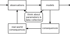
Although our approach is unusual in its use of tools from logic and semantics, the modelling methodology is simply that of classical applied mathematics and simulation, as illustrated in Figure 1. Note

observations models

consequences real-world

consequences think about parameters & data collection

Figure 1: The Classical Modelling Cycle

that we emphasize the importance of integrating the exploration of the parameter space with the construction of models.

In Section 2, we explain the semantic structures that provide the ba-sis for our approach to systems modelling. It is organized according to the distributed systems-inspired view described above. Then, in Section 3, we described the (simplified) class of models that we implement, and explain how this implementation is achieved in the julia language [19]. Then, in Section 3.4.1, we explain how agents and their decision-making are captured in our implemented mod-els, and also consider how system managers’ utility functions can be used to assess the value of policies in both stand-alone and com-posite models.

To illustrate our methods, we base our examples on three models. First, we look at access control to a building and consider the prob-lem of tailgating at the entrance barrier. Second, we consider how employees within an organization decide how to share confidential documents. Third, we consider loss of devices containing confi-dential information by an organization’s employees. Having estab-lished these three models, we then illustrate a key feature of our approach; that is, composition. We show how these models, and their experimental simulations, can be composed to yield a model of information loss from an organization that has access control to its building and a document-sharing policy. In Section 5, we ex-plore experimentally some key properties of these three models.

We provide, in Section 6, a summary of the key features of our work and give a brief discussion of some research directions, primarily concerned with model checking via a modal logic that is naturally

associated with our modelling approach.

Throughout this short paper we seek to maintain an informal, con-ceptual style of presentation. Much of the required underlying mathematics, when presented in full detail, is both quite abstract and quite complex to articulate. Here our primary concern is to articulate a methodology—incorporating structural, economic, and computational aspects—and its use as a tool to support policy decision-making. Accordingly, we aim to give just enough of the mathemat-ical and, indeed, implementation detail to support an explanation of the story. Many readers will have sufficient familiarity with logic, process algebra, and stochastic and experimental methods to ap-preciate what would be required for full detail to be provided. The underlying mathematical set-up as sketched in Section 2.

2. A SEMANTIC BASIS

We give a brief summary of the process-theoretic and logical the-ory that underpins the semantics-based approach to modelling and simulating systems security policy that we have described above. This work is developed in detail in [7, 8, 9].

2.1 Processes and Resources

Milner’s synchronous calculus of communicating systems, SCCS [21], perhaps the most basic of process calculi, provides our first point of departure. This, together with the theory of resources pro-vided by the semantics of bunched logic [22, 9], provides the basis for a calculus of resources and processes. The key components for our purposes are the following:

• A monoid of actions,Act, with a compositionabof elements

aandband unit1;

• The following grammar of process terms,E, wherea2Act

andXdenotes a process variable:

E::=a:E|X

i2I

Ei|E⇥E|X |fixiX.E|(⌫R)E

Most of the cases here, such as action prefix, sum, concurrent prod-uct, and recursion (in thefixicase,XandEare tuples, and we take

theith component of the tuple), will be quite familiar to theorists. The term(⌫R)E, in whichRdenotes a resource, is called hiding, and is available because we integrate the notions of resource and process; it generalizes restriction.

Our notion of resource—which encompasses natural examples such as space, memory, and money—is based mathematically on or-dered, partial, commutative monoids (e.g., the non-negative inte-gers with the monoid of addition with unit zero and order less-than-or-equals), and captures the basic properties of resources discussed briefly in Section 1: each type of resource is based on a basic set of resource elements, which can be combined (and the combination has a unit) and compared. Formally, we take preordered, partial commutative monoids of resources,(R, ,e,_v), whereRis the carrier set of resource elements, is a partial monoid composition, with unite, andvis a preorder onR.

The basic idea is that resources,R, and processes,E, co-evolve,

R, E a_!R0_{, E}0_{, according to the specification of a partial}

‘modi-fication function’,µ: (a, R)_7!R0_{, that determines how an action}

Home

Public Transport

Car

Outside Lobby

Reception

Entryway Atrium Office

Security Guard Access Control

forgot badge?

choice

observed tailgating? tailgate

choice

challenge

ignore caught?

challenged?

yes

caught? challenged? tailgate

no

search for send document

choice

lose device? Employee

Attacker

Outside Atrium

to Entryway to Atrium

queue for badge

yes

no

Attacker

ENV ENV

yes no

to Atrium wait...

wait... wait...

ENV

ENV

work to Outside

travel

Composed Composed

Composed

Composed

Composed Employee

Employee

no

yes

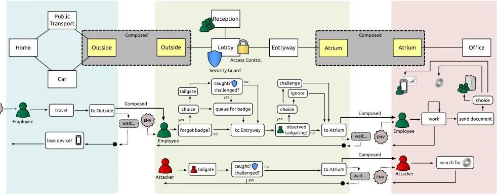
Figure 2: A depiction of the three example models, showing their locations and processes, and how the models are composed together

The base case of the operational semantics is given by action prefix:

R, a:E a_!R0_{, E} µ(a, R) =R 0_.

Concurrent composition,⇥, exploits the monoid composition, , on resources,

R, E !a R0, E0 S, F !b S0, F0

R S, E⇥F ab!R0 _S0_{, E}0_⇥F0.

Modification functions are required to satisfy some basic coher-ence conditions: µ(1, R) = R, where1is the unit action, and, ifµ(a, R) µ(b, S)andR Sare defined, thenµ(ab, R S) '

µ(a, R) µ(b, S), where'is Kleene equality, for all actionsaand

band all resourcesRandS. In certain circumstances, additional equalities may be required [7, 9].

Sums and recursion are formulated in familiar ways:

R, Ei !a R0, E0 R,P_i2IEi a!R0, E0

and R, Ei[E/X]

a

!R0, E0 R,fixiX.E a!R0, E0

,

whereIis an indexing set andEiis theith component of the tuple Eof processes. Other combinators are handled similarly.

2.2 Location

Just as our treatment of resources begins with some basic obser-vations about some natural and basic properties of resources, so we begin our treatment with the following basic requirements of a useful notion of location [9], including a collection of atomic locations—the basic places—which generate a structure of loca-tions, and a notion of (directed) connection between locations— describing the topology of the system.

We can also consider a notion of sublocation (which respects con-nections) and a notion of substitution (of a location for a subloca-tion) that respects connections—substitution provides a basis for abstraction and refinement in our system models. The notions of sublocation and substitution are intimately related, the former be-ing a prerequisite for the latter. We do not develop or support sub-stitution in the current version of our implemented models.

We remark briefly that treating location as a first-class citizen in this way does not lead to a process calculus with operational behaviour that is more expressive in absolute terms. It does, however, lead to greater pragmatic expressiveness and simplifies the construction of models of a wide range of systems.

The resulting calculus has a transition system given by a judge-ment of the formL, R, E a_!L0, R0, E0, whereais an action (in the usual process sense),L,L0are location environments,R,R0

are resource environments andE, E0 _{are processes used to}

con-trol the evolution. As sketched above, we define a modification function, µ, which, for each actiona, location L, and resource

R, determines the evolved locationL0 and resourceR0: that is, µ: (a, L, R) _7!(L0_{, R}0_{), with corresponding versions of the}

co-herence conditions. In a stateL, R, E, the componentLcarries the relevant information about the topology of the model andR

car-ries the relevant information about the distribution of the resources around the model’s topology.

The operational semantics extends to locations very naturally. The following is the rule for action prefix:

L, R, E a!L0_{, R}0_{, E}0 (L

0_{, R}0_{) =µ(a, L, R)}

The details of the operational semantics with location and its im-plementation may be found in [9].

2.3 Environment

The systems that we model do not exist in isolation, but rather in-teract with an environment that we choose not to model in detail. Rather, we represent an environment by capturing the incidence on the model of events from the environment stochastically. For ex-ample, the arrival rate of agents at entrance that marks the outer boundary of a model may be captured using a negative exponential distribution [24, 18]. Similarly, a model may capture outputs from the system that is modelled to the surrounding environment.

2.4 Gnosis: A Proof-of-concept Tool

The semantic basis for system modelling described above has been implemented in a proof-of-concept modelling tool called Gnosis [8, 9] that closely captures the semantic structure of processes, re-sources, and locations. In [8, 9], a formal semantics of Gnosis is given in the semantic structures described above. Since the stochas-tic aspects of models are not captured directly in these structures, Gnosis’s scheduler is given a denotational definition within them.

In the implementation described in this paper, we employ not Gno-sis, but rather a new framework written in julia [19]. julia is well-adapted to describing the simplified implemented models that we explain in detail in the next section and is supported by well-engin-eered programming and graphics environments. Our use of julia is explained in Section 3.4.

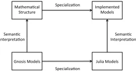
The relationship between the abstract semantic structures for pro-cesses, resources, and locations, the implemented models, Gnosis models, and julia models can summarized by the following dia-gram: Each of the arrows can be given a precise mathematical

def-Mathema'cal*

Structure* Implemented*Models*

Gnosis*Models* Julia*Models*

Seman'c*

Interpreta'on* Interpreta'on*Seman'c*

Specializa'on*

Specializa'on*

inition; for example, the interpretation of Gnosis models in the se-mantic structures is spelled out in [8, 9], and the interpretation of julia models in our implemented models is similar.

3. IMPLEMENTED MODELS

The mathematical structure of models as described above provides the basis for the class of models that we implement. We employ well-motivated simplifcations of the general semantic set-up.

Figure 3: The basic structure of implemented models

Models in this methodology are designed to be composed with other models (Figures 3 and 4). Composition allows us to join two or more models together and see what effects their interaction has. When models are composed there are interactions at the location, process, and resource levels, and the role of their intended envi-ronments is critical. Processes transition and resources are moved between models at locations shared between the models.

Interface)

Figure 4: The basic structure of composed models

To enable composition, models contain interfaces, which define the locations where models fit together and which actions, defined at appropriate locations within the interface, are party to the compo-sition. Actions in the interface will nevertheless be able to execute only if the resources they require are available.

3.1 Definitions of Implemented Models

The locations and resources of a model are represented using a lo-cation graph,G(_V[_R],_E), with a set of vertices,V, representing the locations of the model, and a set of directed edges,E, giving the connections between the locations. Vertices are labelled with resourcesR.

As explained above, actions evolve the processes and resources of a model. However, rather than thinking of actions evolving pro-cesses, it is convenient to think of a process as a trace of actions— the history of actions that have evolved a process during the execu-tion of the model. All of the acexecu-tions in a model are contained in a set,A, and process traces are comprised of these.

The environment a model sits inside causes actions within the model to be executed, at a particular location. A model contains a set of lo-cated actions,L, and a located action,l_2L, is given by an ordered pairl= (a2A, v2V). The environment associates these located

actions with probability distributions: Env : _{L !} P robDist. During the execution of the model, the located actions are brought into existence by sampling from these distributions.

Models also need to have interfaces in order to support composi-tion. An interfaceI_2Ion a model is a tuple(In, Out, L)of sets of input and output vertices, whereIn✓VandOut✓V, and a set of located actionsL_✓L.

The sets of input vertices and output vertices in interfaces must be disjoint; that is

\

i2I

Ini2In=; and

\

i2I

Outi2Out=;.

DEFINITION 1. A modelM = (_G(_V[_R],_E),_A,_P,_L,_I)is a tuple that consists of a location graphG, a set of actionsA, a set of processesP, a set of located actionsL, and a set of interfacesI.

3.2 Composition of Implemented Models

Two models, M1 and M2 are composed with specific interfaces

I1,1, . . . , I1,j, . . . , I1,n 2 I1 andI2,1, . . . , I2,k, . . . , I2,m 2 I2

using the composition operator,M1I1,j|I2,kM2, which is defined

using an operation, , on each of the elements of a model.

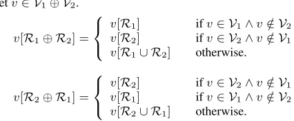
First, we define the operator for vertices and edges,

V1 V2=V1[V2

and, for eachv2V1 V2,

v[R1 R2] = 8 < :

v[R1] ifv2V1^v /2V2

v[_R2] ifv2V2^v /2V1

v[_R1[R2] otherwise.

.

Composition of edges, actions, and proceeses are straightforward:

E1 E2=E1[E2,A1 A2=A1[A2, andP1 P2=P1[P2.

tuples; for example, the interfaces ofM1:I1={(In1, Out1, L1)i}.

A particular interface fromI1 is referred to asI1,i, and the input

locations from that interface are referred to asIn1,i, the outputs as Out1,i, and the located actions asL1,i.

When models are composed, the located actions in the interface that were executed by the environment in the uncomposed model are now executed as a consequence of the other model instead. As such, the composition of located actions is the union of both sets of located actions, minus those that are in interfaces used in the composition:L1 L2=L1[L2\ {L1,j, L2,k}.

Interfaces can be used in just one composition, and the input and output locations of the interfaces from the two models must corre-spond, so their composition isI1 I2= (I1[I2)\ {I1,j, I2,k},

where we requireSn

j=1InI1,j=

Sm

k=1OutI2,kand

Sn

j=1OutI1,j =Sm_k=1InI2,k. Models must be composed completely: any

loca-tion that is in both of the models must belong to the interfaces used in the composition.

DEFINITION 2. With the data as established above, the

compo-sition of modelsM1andM2is given by

M1I1,j|I2,kM2 = (G((V1 V2)[R1 R2],E1 E2),

A1 A2,P1 P2,L1 L2,(I1 I2)), with the constraint thatV1\V2=In1,j[In2,k.

PROPOSITION 1. M1I1,j|I2,kM2is a model.

PROOF. The composition of each of the components of the mod-els is well-defined:

• G1 G2((V1 V2)[R1 R2],E1 E2)is immediately a

location graph with verticesV1[V2, resourcesR1 R2,

and edgesE1[E2;

• A1 A2andP1 P2are trivially the unions of the actions

and processes, respectively;

• L1 L2is trivially a set of located actions.

The sets of input vertices and output vertices in the composed model must both be disjoint. With the constraints thatV1\V2=In1,j[ In2,kand thatSn_j=1InI1,j =

Sm

k=1OutI2,kand

Sn

j=1OutI1,j =

Sm

k=1InI2,kthen any locations in both of the models are present

in the interfaces used for composition and(I1[I2)\ {I1,j, I2,k}

is a well-defined set of interfaces.

PROPOSITION 2. Composition of models is commutative:

M1I1,j|I2,kM2=M2I2,k|I1,jM1

PROOF. Each component of the model is commutative.

Trivially,A1 A2=A2 A1,L1 L2=L2 L1, andP1 P2=

P2 P1.

Next, location graphs:G1 G2((V1 V2)[R1 R2],E1 E2) = G2 G1((V2 V1)[R2 R1],E2 E1). The edges are

straight-forward: E1 E2 = E2 E1. Vertices are trivial—V1 V2 = V2 V1—but resources require more care:(V1 V2)[R1 R2] =

(V2 V1)[R2 R1].

For resources, we must show that anyv_2V1 V2gets the same

assignment of resources fromR1 R2asR2 R1.

Letv2V1 V2.

v[_R1 R2] = 8 < :

v[_R1] ifv2V1^v /2V2

v[_R2] ifv2V2^v /2V1

v[R1[R2] otherwise.

v[_R2 R1] = 8 < :

v[R2] ifv2V2^v /2V1

v[_R1] ifv2V1^v /2V2

v[_R2[R1] otherwise.

For the remaining case,v[_R1[R2] = v[R2[R1]. In the other

cases, thenvis either inV1orV2so, regardless of order,v[R1 R2] =v[R2 R1] =v[R1]ifv2V1andv[R2]ifv2V2.

Finally, interfaces:I1[I2=I2[I1and{I1,j, I2,k}={I2,k, I1,j},

soI1 I2=I2 I1. We know from Proposition 1 that the

com-position of interfaces is well-defined.

For any pair of modelsM1andM2, letI1!2 be the subset of

in-terfaces inI1that compose withM2.

PROPOSITION 3. Composition of models is associative:

(M1I1!2|I2!1M2)I1!3[I2!3|I3!1[I3!2M3

=

M1I1!2[I1!3|I2!1[I3!1(M2I2!3|I3!2M3)

PROOF. The proof unpacks the definition of composition in a

style similar to the proof of Proposition 2. The details are straight-forward.

3.3 Environment

As we have previously explained, in Section 2.3, the environment represents things outside the scope of the model: events and de-tails that have an effect on the model, but are too complicated or of not enough interest to model directly. The modeller chooses a distribution to represent the likelihood of these events occurring, and these distributions are sampled to determine when to execute located actions within the model.

When models are composed, some of these located actions are re-moved, meaning that the distributions previously chosen for them are not sampled and the actions are no longer a consequence of the environment. Instead, the located actions are initiated by a process in the other model, but they are still, at some level, dependent on the environment because the other model still samples from it.

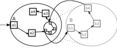
Consider Figure 5, which shows two processes,AandB, from two different models, which are represented as a sequences of actions:

A = input _! a1, a2, a3, a4 _! outputand B = input _! b1, b2, b3, b4.

a1

a2 a3 _a4

b1 b2

b3 b4

A

Figure 5: Models with processes started by the environment

might look like Figure 6. The sequence of actions is nowinput!

a1, a2, a3, a4, b1, b2, b3, b4

a1

a2 a3 _a4

b1 b2

b3 b4

Figure 6: The two models have been composed. The second process is started by the first instead of the environment

Now, only one process is started by the environment. What was once the second process,B, is now started at the end ofA.

A more complicated example occurs when the composition does not occur at the end of a process. In this case, the initial processes are shown in Figure 7. The sequence of actions for process A is

A=input_!a1, a2, delay, a3, a4_!outputand the sequence for process B isB=input_!b1, b2, b3, b4_!output.

a1 a2

a3 a4

b1 b2

b3 b4 A

delay

B

Figure 7: Two models with processes started by the environ-ment. Process A has a special action,delay

InA, there is a special action,delaywhich is where composition would occur. In an uncomposed executing model, this stops the process for a period of time before continuing. When composed, the process looks like Figure 8. The sequence of actions is now

input_!a1, a2, b1, b2, b3, b4, a3, a4_!output.

a1

a2 a3 a4

b1 b2

b3 b4

A _B

b1 b2

b3 b4

Figure 8: The two models have been composed. Process B has now been substituted for thedelayaction in process A

The delay in processAsimulates the time that would have elapsed if the model were more detailed. This detail is present in the com-posed model and so the delay is no longer needed.

3.4 Implementation in julia

The modelling framework is implemented in the julia language, a new language designed for scientific computation. The models are then also written in julia, on top of this framework. The features of the language make it relatively straightforward to implement the concepts required for modelling.

Processes, for example, are represented naturally with julia’s Tasks— commonly known as coroutines. In combination with a scheduler, this allows processes to run, wait for a period of time, and resume execution. In the example below, the very simple process starts, suspends for 5 hours of simulation time, and then terminates.

f u n c t i o n e x a m p l e _ p r o c e s s ( p r o c : : P r o c e s s ) h o l d ( proc , 5 h o u r s )

end

Resources are simply types in julia that are subtypes of the ab-stractResourcetype. For example,Agentis an abstract sub-type ofResourceandEmployeeis a subtype ofAgent. The

Employeetype has a field,data, which is used for storing infor-mation about this agent: preferences, what it is carrying, etc.

a b s t r a c t Agent <: Resource t y p e Employee <: Agent

d a t a : : AgentData end

Locations are created and then linked together. l o c a l l o c _ a t r i u m = L o c a t i o n ( " Atrium " ) l o c a l l o c _ o f f i c e = L o c a t i o n ( " O f f i c e " ) l i n k ( l o c _ a t r i u m , l o c _ o f f i c e )

In addition to these basic elements, the framework also comprises a library of useful components, such as doors, access control mecha-nisms, and function libraries useful for building new models.

3.4.1 Agents

Each agent in the system is modelled using bundle of a process, a resource, and one or more locations. The resource marks the agent’s physical location in the model. The agent’s process moves this resource between the locations in the model, and also inter-acts with other resources as needed. The locations bundled with the agent are used to model concepts like holding or remembering. To model an agent picking up another resource, the agent’s pro-cess would move that resource into the location that represents the things the agent is carrying; dropping the resource would move it back to a physical location in the model.

3.4.2 Agent Decision Making

In addition to moving around and interacting with resources, agents must also make decisions. These decisions occur at specific points in the agent’s process and the agent decides between a number of alternative choices. In theory, any method may be used to decide between the choices, but in practice the decision is based on the current state of the model and the agent’s preferences.

In these models, we use a straightforward approach to decision-making: for each choiceC, the agent calculates

val(C) =psecfsec(C) +pprodfprod(C)

wherepsecandpprodare the agents preferences towards security

and productivity, respectively. The functionsfsec(C)andfprod(C)

determine the current value to the agent, based on the state of the model, of the choiceCin terms of security and productivity. The agent then selects the highest valued choice.

The agent’s preferences for security and productivity are drawn stochastically from distributions at the start of the execution of the model. The distributions should be chosen to reflect the population of agents in the system being modelled.

3.4.3 Composition

The first interface is for the Outside location, where the model com-poses with the device loss model. This is an input location—a process is started from the other model rather than the environ-ment, when composed. The code creates the interface, then the input location, sets an environment processes responsible for start-ing the agents in the model when it is not composed, and defines which function should be executed from another model when com-posed with this model. Theagent_process function corre-sponds to a located action in the mathematical definition of an in-terface above. The environment process,start_agents corre-sponds to the mapping of a probability to a located action; in fact, the function just callsagent_processfor each agent at random times drawn from a distribution.

i f a c e _ o u t s i d e = I n t e r f a c e ( ) i l = I n p u t L o c a t i o n ( )

push ! ( i l . e n v _ p r o c e s s e s ,

P r o c e s s ( " s t a r t _ e m p l o y e e s " , s t a r t _ a g e n t s ) ) i l . f u n c t i o n s [ Agent ] = a g e n t _ p r o c e s s

i f a c e _ o u t s i d e . i n p u t _ l o c a t i o n s [ " O u t s i d e " ] = i l model . i n t e r f a c e s [ " O u t s i d e " ] = i f a c e _ o u t s i d e

i f a c e _ a t r i u m = I n t e r f a c e ( ) o l = O u t p u t L o c a t i o n ( )

o l . f u n c t i o n s [ Agent ] = i n _ a t r i u m

i f a c e _ a t r i u m . o u t p u t _ l o c a t i o n s [ " Atrium " ] = o l model . i n t e r f a c e s [ " Atrium " ] = i f a c e _ a t r i u m

push ! ( model . e n v _ p r o c e s s e s ,

P r o c e s s ( " s t a r t _ a t t a c k e r s " , s t a r t _ a t t a c k e r s ) )

Figure 9: Code for creating interfaces in the tailgating model

The second interface is for the Atrium location, where the tailgating model composes with the document-sharing model. It is an output location: the agent and attacker processes from this model continue into the document-sharing model when it is composed. When not composed, the processes execute thein_atriumfunction as set in the code. This function just pauses the processes for a set amount of time—it is thedelayaction from above. When composed, the actions in the other model are executed instead of this.

Finally, composition itself is similar to the mathematical definition. Thecomposefunction takes two models and specified interfaces and returns the composed model. Figure 10 shows the code for composing all three of the models together. First the device loss and tailgating models are composed together, and then the resulting model is composed with the document-sharing model.

4. SYSTEM MANAGERS’ UTILITY

This modelling methodology is designed to allow system managers to explore the effects and consequences of various policy decisions on a a system. A necessary component of this is the ability to

ex-m1 = c r e a t e _ d e v i c e _ l o s s _ m o d e l ( ) m2 = c r e a t e _ t a i l g a t i n g _ m o d e l ( ) m3 = c r e a t e _ d o c u m e n t _ s h a r i n g _ m o d e l ( )

temp_m = compose (m1 , " O u t s i d e " , m2 , " O u t s i d e " ) m = compose (m3 , " Atrium " , temp_m , " Atrium " )

Figure 10: Code for composing the three models together

press how good the performance of a system is given certain par-ticular policy choices and the system manager’s preferences.

We can express this value—the utility of a policy choice—in terms of a set of attributes that the system manager cares about [17, 20]:

U tility=X

a2A

wafa(va v¯a)

Each attribute,a, has a functionfathat determines the system

man-ager’s response to the deviation of the value of the attribute,vafrom

its target value,¯va. For example, for one attribute the system

man-ager might not care about missing the target by a small amount, but for another attribute a small deviation from the target could be crit-ical. Each attribute also has a weighting,wa, describing its relative

importance compared to others. When models are composed, the overall utility simply adds together the component utilities.

The target values, weightings, and deviation functions for the at-tributes are obtained from the system manager. To evaluate the performance of current policy, the values for each of the attributes can be obtained from the real world. To evaluate changes to policy, the values of the attributes can be obtained from models.

The values of the attributes can depend on the decisions that agents make during an execution of the model. A decision,D, made by

an agent can be written in Cobb-Douglas form [15] as

D=C 1

1 C22. . . Cnn

whereC1, C2, . . . , Cnare the values to the system manager of the

choices available for that decision. The exponents 1, 2, . . . , n

take the value0for the choices not selected, and the value1for the

choice that was selected.

Each agent makes a series of decisions as the model executes, and the set of the decisions made by all of the agents during the exe-cution of a model can be used when calculating the values of the attributes in the system manager’s utility function. Once those val-ues have been obtained, the utility for that execution of the model can be determined.

4.1 Expected Utility

Knowing the utility of a single execution of a model is not that useful if the model contains stochastic elements—it is just one of many possible outcomes. Instead, we must find the expected utility

E[U tility] =E "

X

a2A

wafa(va( a) v¯a)

#

where the expected value for each attributeadepends on the stochas-tic process a. Again, expected utilities for composed models

sim-ply add those of the components.

The values of these processes also depend on the decisions indi-vidual agents make. However, we need to consider the expected value of these decisions to account for all possible outcomes. This means that the values are no longer0or1, indicating the choice made during a single execution of a model, but rather probabili-ties giving the likelihood of each choice being made. A standard transformation of the Cobb-Douglas form [25] gives

E[D] = 1ln(C1) + 2ln(C2) +· · ·+ nln(Cn)

where 1, 2, . . . , nare now the probabilities of the agent

These probabilities, along with each a, depend on the state of the

model, which in turn depends on stochastic elements of the model and its environment. In theory, these values can be calculated start-ing with the known probability distributions and usstart-ing queuestart-ing theory to work out the subsequent states of the model. In prac-tice, this is extremely difficult and an approximation of these values must be used. This is done by executing the model a large number of times, to get an approximate distribution of values. The accuracy of this estimation increases with the number of executions.

5. MODELS AND EXAMPLES

5.1 Models

We will use three different models that examine different areas of security policy as examples. The first of these models is a tailgat-ing model, which looks at the behaviour of employees and attack-ers at the entrance to an office building. The second model looks at the behaviour of employees inside the office, when they are mak-ing decisions about how to share confidential documents with other employees. The final model is extremely simple, and looks at the loss of devices, possibly containing confidential data, outside of the office. These three models are depicted in Figure 2.

5.1.1 Tailgating

The tailgating model looks at how different security policy choices at the entrance to the building affect the behaviour of employees and attackers. This model is shown in the centre of Figure 2. In the model, employees need an ID card in order to get through the security door. When employees forget their cards, they must make a decision: to queue at the reception desk to get a temporary ID card for the day, or to tailgate through the door. Employees that have passed through the security door observe if others tailgate behind them; if so, the employee has another choice: to ignore the tailgater and continue straight to the office, or to stop the tailgater and send them back to reception. There are also attackers in this model, who always try to tailgate and do not have any decisions. They can be stopped by security guards and by employees’ challenges.

5.1.2 Document Sharing

The document-sharing model looks at the behaviour of employees inside the office when they must decide how to share confidential documents with each other. This model is shown on the right side of Figure 2. Normally, employees share documents using a shared drive that restricts access to each document to employees with the appropriate authorization. However, the system is often unavail-able and employees must use an alternative means to share the doc-uments. In the model, there are three choices. First, is to use a global share, which is accessible by all employees. Second, is to email the documents to the recipients. Finally, employees can use portable media, such as a CD or USB stick to share the data. Each of the three options has a drawback: documents on the global share can be accessed by any employee, documents sent to email end up on the devices which employees carry to and from work, and the portable media used to share documents gets left lying around the office. In this model, attackers walk around the office and pick up any portable media they find lying around.

5.1.3 Device Loss

The device-loss model is very simple: employees that return home from work have a random chance to lose devices they are carrying, which possibly contain confidential data. By itself, this model does not do very much. When composed, however, it becomes more

useful: the number of confidential documents on the devices is de-termined by the behaviour of employees in the document-sharing model. This model is shown on the left side of Figure 2.

5.1.4 Composed Model

The three models are designed to compose together at specific in-terfaces. The Outside locations in the device-loss model and the tailgating model are part of the interfaces for those models. When composed, the models are joined at that location. The same is true for the tailgating model and the document-sharing model: they are composed at the Atrium location in each of the models.

Some of the processes in each model are also part of the compo-sition. When the tailgating model is not composed, the Employee processes are started by the environment, and agents that make it through to the Atrium simply wait there for the duration of the work day before leaving. When the model is composed to the device loss model, the Employee processes start in that model, and then con-tinue to this one. When the tailgating model is composed with the document-sharing model, the employee and attacker processes in the document-sharing model are executed as consequences of the tailgating model, rather than started by the environment.

5.1.5 Validation

The parameters used in our experiments have been chosen to illus-trate our methodology simply and clearly. However, the formula-tion of each of the example models is based directly upon extensive empirical studies of organizational behaviours (e.g., both employ-ees and managers) in a large critical infrastructure company. More-over, the experimental results of the simulations closely match ob-served behaviours in the parts of the company upon which the ex-ample scenarios are based.

5.2 Examples

We will use two fictional companies with different attitudes to-wards security for our examples. The first company places a high value on security and the confidentiality of its information; this could be a corporate research lab in a competitive field, or a na-tional infrastructure company. The second company values secu-rity much less, and is more concerned with allowing people to get work done than keeping information secret.

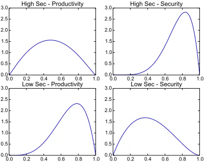
The different attitude towards security in these companies is present in both the preferences of the employees and those of the organi-zations’ security managers. In these examples, the distributions of employee preferences are chosen to reflect what is likely to be found in the respective companies. In reality, these distributions would be determined by sampling the preferences of actual em-ployees at the organizations. The distributions we are using are shown in Figure 11. The highly-secure company contains employ-ees who for the most part value security very highly over productiv-ity. In the lower-security company, the employees are more likely to have a higher preference for productivity than for security.

Figure 11: PDFs of employee preference distributions

Table 2 shows the results for the document-sharing model. In the high-security company, employees have high preferences for secu-rity; most follow the instructions to use either email or portable me-dia. In contrast, employees in the low-security company are much more concerned with productivity; the instructions have little ef-fect. This shows how the security culture of a company and its em-ployees can have an effect on the performance of policy. A more complete presentation of simulation results would include confi-dence intervals for the values.

Company a wa v¯a fa(x)

High Sec Share 0.25 20 (e0.01x_{+ 0.01x 1)}

Found 1 0 ex_{+ 1}

Lost 1.1 0 ex+ 1

Rcpt Time 0.01 3000 -.002x

Tgate 1.5 0 ex_{+ 1}

Low Sec Share 0.1 200 .003x

Found 0.3 0 ex_{+ 1}

Lost 0.4 0 ex_{+ 1}

Rcpt Time 0.4 2000 -.005x

Tgate 0.2 0 ex_{+ 1}

Table 1: Utility parameters

The weights, targets, and deviation functions for each attribute used in the utility calculations are shown in Table 1. For the document-sharing model, only the first two attributes (the number of ments on the globally accessible share and the number of docu-ments on portable media found by attackers in the office) are used. The security managers of the high and low security companies have different weightings, targets, and deviation functions. The high se-curity manager is trying to reduce the number of documents shared globally and so has a low target value. A Linex function [26] is used for the deviation function for this attribute: beating the tar-get results in a linear increase in utility; missing it results in an exponential loss. The low security manager actually prefers that employees use the global share as it is more efficient and confiden-tiality is not an issue. Both managers have an exponential response to attackers finding documents on portable media inside the office, but have different weightings.

In this case, the high-security manager would prefer the email pol-icy, as it produces the lowest number of documents on the global share, and does not leave media devices lying around the office to be found by attackers. The low-security manager prefers no change of policy: employees should keep using the global share.

Company Policy Email Share Media Found E[U]

High Sec Email 151.73 7.75 0.00 0.00 0.059 None 0.00 167.32 0.00 0.00 -1.209 Media 0.00 54.42 105.33 2.43 -10.543 Low Sec None 0.00 167.29 0.00 0.00 -0.010 Email 54.87 107.96 0.00 0.00 -0.028 Media 0.00 154.15 12.24 0.07 -0.035

Table 2: Results from the document-sharing model

The managers would like to know that these policies are still opti-mal when considered as part of the larger system. Composing the document-sharing model with the tailgating and device loss models allows the managers to see the interactions between policy choices in each model. In the tailgating model, the managers must choose the number of security guards and receptionists, which can affect how many attackers gain access to the office. The managers also care about more attributes from the other two models: the number of documents on lost devices, the number of times attackers suc-cessfully tailgate, and the amount of time employees spend at re-ception. The weightings, targets, and functions for these attributes are shown in Table 1. The high security manager cares less about the time taken at reception and more about the number of tailgates and devices lost. In contrast, the low security manager cares more about reducing the time employees spend at reception.

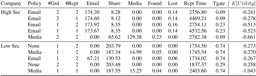
Table 3 shows the results from the composed model for some pa-rameter combinations. For the high-security manager, the email policy is still the best option as long as there is at least one guard. The difference in expected utility between the email and media policies is much smaller than in just the document-sharing model as the guards and challenges by employees prevent attackers from accessing the office. For the low-security manager, having two re-ceptionists is the most important factor: it greatly reduces the time employees spend at reception. Using two guards instead of one ac-tually results in less expected utility, as the guards catch more em-ployees tailgating, who must then spend the time at reception. The influence of employee preference can be seen again in this com-posed model: for the same number of guards in the low- and high-security companies, there are more tailgates in the low-high-security company because the employees do not challenge tailgaters.

6. CONCLUSIONS AND FURTHER WORK

We have presented a rigorously grounded, compositional modelling framework and methodology capable of capturing the consequences and values of systems security policy design decisions. We have demonstrated this framework in some simple, but empirically sup-ported, examples of concern to practising security managers that illustrate all aspects of the methodology and its value in supporting their decision-making.

Company Policy #Grd #Rcpt Email Share Media Found Lost Rcpt Time Tgate E[U tility]

High Sec Email 2 2 174.20 8.28 0.00 0.00 0.14 2756.80 0.09 -0.241 Email 2 1 174.60 8.12 0.00 0.00 0.14 4469.21 0.09 -0.278 Email 1 2 173.92 8.35 0.00 0.00 0.16 2754.11 0.23 -0.513 Email 1 1 173.67 8.35 0.00 0.00 0.14 4532.56 0.23 -0.523 Media 2 2 0.00 65.62 129.38 0.23 0.00 2782.38 0.09 -0.661 Low Sec None 1 2 0.00 203.79 0.00 0.00 0.00 1754.50 0.74 0.273 Media 1 2 0.00 187.34 14.99 0.05 0.00 1745.54 0.74 0.270 Email 1 2 67.21 130.53 0.00 0.00 0.06 1734.02 0.74 0.267 None 2 2 0.00 203.48 0.00 0.00 0.00 1837.37 0.29 0.258 Media 1 1 0.00 187.55 15.25 0.04 0.00 2403.60 0.74 -1.043

Table 3: Results from the composed model

Concerning experimental methodology, we need to develop a more systematic approach to analyzing the sensitivity of model execu-tions and utility to parametrization choices [18]. More generally, a systematic methodology for exploring how managers’ elicited pref-erences [1, 4] can be represented in model structure and parametriza-tion should be explored.

Associated with the process-algebraic tools described in Section 2 is a modal logic, in the tradition of Hennessy–Milner logic [16, 9], in which propositions assert properties of system states. The logic is given semantically by a satisfaction relation,L, R, E_|= , inductively defined over the logic’s connectives, and read as ‘the processE, executing at locationLwith available resourcesRhas property ’. The logic’s connectives include additives and plicatives of the bunched logic BI [22] and both additive and multi-plicative modalities [9], so rendering it capable of expressing both structural and dynamic properties of models. Model checking— with some initial work described in [9], but much more work requir-ed—would provide a framework within which stateful properties of systems, as well as utility-theoretic properties of policies, such as optimality, can be verified. A further step would be to incorporate the stochastic aspects of implemented models into model-checking tools, perhaps building on ideas in, for example, PRISM [23].

7. REFERENCES

[1] AI Magazine: Preferences. J. Goldsmith and U. Junker

(editors). Volume 29, No 4, Winter 2008. [2] A. Beautement et al.. Modelling the Human and

Technological Costs and Benefits of USB Memory Stick Security. InManaging Information Risk and the Economics of Security, M. Eric Johnson (ed.), Springer, 2008. 141–163. [3] A. Beautement, M. Angela Sasse, and M. Wonham. The

Compliance Budget. Proc. New Security Paradigms Workshop, 2008 (NSPW ’08), 47–58. ACM New York, 2008. doi: 10.1145/1595676.1595684

[4] Y. Beres, D. Pym, and S. Shiu. Decision Support for Systems Security Investment. InProc. Business-driven IT

Management (BDIM), IEEE Xplore, 2010, 118–125. doi:

10.1109/NOMSW.2010.5486590

[5] T. Caulfield, D. Pym, and J. Williams. Compositional Security Modelling: Structure, Economics, and Behaviour. LNCS 8533:233–245, 2014.

[6] J. Cohen, S. McClure, and A. Yu. Should I stay or should I go? How the human brain manages the trade-off between exploitation and exploration.Phil. Tran. Roy. Soc. B: Biol. Sci.362(1481), 933–942, 2007.

[7] M. Collinson and D. Pym. Algebra and logic for

resource-based systems modelling.Mathematical Structures

in Computer Science19:959-1027, 2009.

[8] M. Collinson, B. Monahan, and D. Pym. Semantics for structured systems modelling and simulation.Proc.

SIMUTools 2010, 34:1–34:10. ACM Digital Library.

doi:10.4108/ICST.SIMUTOOLS2010.8631

[9] M. Collinson, B. Monahan, and D. Pym.A Discipline of

Mathematical Systems Modelling.College Publications,2012.

[10] Core Gnosis.http://www.hpl.hp.com/research/ systems_security/gnosis.html.

[11] G. Coulouris, J. Dollimore, and T. Kindberg.Distributed

Sy-stems: Concepts and Design. Addison Wesley, 3rd ed., 2000.

[12] C. Fang and D. Levinthal. Near-Term Liability of Exploitation: Exploration and Exploitation in Multistage Problems.Organization Science20(3), 538–551, 2009. [13] L. Gordon and M. Loeb. The Economics of Information

Security Investment.ACM TISSEC, 5(4):438–457, 2002. [14] L. Gordon and M. Loeb.Managing Cybersecurity

Resources: A Cost-Benefit Analysis. McGraw Hill, 2006.

[15] D. Heathfield.Production Functions. MacmillanPress,1971. [16] M. Hennessy and G. Plotkin. On observing nondeterminism

and concurrency. LNCS 85, 299–309, 1980.

[17] C. Ioannidis, D. Pym, and J. Williams. Information security trade-offs and optimal patching policies.European Journal

of Operational Research216(2):434–444, 2011.

[18] R. Jain.The Art of Computer Systems Performance Analysis. Wiley and Sons, 1991.

[19] julia.http://julialang.org.

[20] R.L. Keeney and H. Raiffa.Decisions with multiple objectives. Wiley, 1976.

[21] R. Milner. Calculi for synchrony and asynchrony.Theoret.

Comp. Sci., 25(3):267–310, 1983.

[22] P. O’Hearn and D. Pym The Logic of Bunched Implications.

Bulletin of Symbolic Logic5(2), June 1999, 215–243.

[23] The PRISM Model Checker.

http://www.prismmodelchecker.org

[24] S. Ross.Introduction to Probability Models. Eighth Edition, Academic Press, 2003.

[25] H. Varian. Intermediate Microeconomics. W.R. Norton & Company, 2014