Critical Slowing Down in Depression: A Case Study
Leonie Seeland
S1723251
Master Thesis Clinical Psychology
Supervisor: Prof. W. Van Der Does, PhD
Institute of Psychology
Universiteit Leiden
Abstract
According to current research, there might be a process of critical slowing down of the
system happening before a depressive episode. This paper investigates whether this can be seen
in the case of a Dutch woman with Major Depressive Disorder. We used the subject’s diary to
investigate whether critical slowing down existed before two selected depressive episodes using
autocorrelation scores of mood variables, as well as sleep, relaxation and physical exercise. We
did not find conclusive evidence for the existence of critical slowing down before the depressive
episodes and there is further research needed to investigate this phenomenon.
Case studies have always been popular among researchers. Early pioneers of psychiatry
like Freud and Kraepelin primarily used case studies to make their points. Big achievements,
such as the theories about fear conditioning or about the role of brain structure on gender roles
were developed or significantly advanced through case studies (Diamond & Sigmundson, 1997;
Watson & Rayner, 1920). On the one hand, there are many advantages in using case studies for
research (Kazdin, 2014). Looking at a single case provides the opportunity to look at the details
which can get lost in big randomized controlled trials. Psychology often is about change, which
can be investigated very closely in a case study. On the other hand, case studies also have
limitations. They do not provide reasonable ground for generalization to the population as there
are only one or few participants, who are not randomly allocated to different conditions, as in
randomized controlled trials. Classical case studies in psychotherapy mostly provided descriptive
data, either from the case themselves or from the researcher, which are often very subjective.
Neuropsychological case studies tend to include test scores, which may or may not be included in
psychotherapy cases. Another limitation of classical case studies is that they cannot provide any
causal indication, as there usually is no control condition included in the research design (Kazdin,
2014).
Several types of case studies exist, which all have their disadvantages and advantages.
Case study reports can present one case but they can also present several individuals in detail or a
group of individuals. Another major distinction can be made between a traditional case study and
an experimental case study (Kazdin, 2014). The traditional, non-experimental case study is
descriptive rather than experimental. Thus, there is often no experimental manipulation, but
rather a description of an individual, community or group. It often, but not exclusively, describes
a case that shows distinctive features from previously known cases. An example for this is the
case of Phineas Gage, which led to new conclusions about the structure of the brain (Harlow,
1848). This case study describes the brain injury of a man named Phineas Gage who suffered
behavioral consequences after an iron rod passed through his skull. This case study is rather
descriptive, as it merely describes the case and its value for the scientific field.
An experimental case study, in contrast, includes a manipulation of some kind to ensure
shifted between the different cases or that the intervention is given and taken away repeatedly
within one subject (see Ter Kuile et al., 2009 for example). A very well-known example for this
would be Skinner’s research on operant conditioning (Skinner, 1938). Skinner designed an
experimental series with rats. Each rat was put in a box which had a lever in it. When the lever
was pushed, nothing happened at first. After a certain time, the rat was given food each time the
lever was pushed. The rate of the rat pushing the lever increased as soon as it has learned that
pushing the lever equals food. Thus it had been conditioned to push the lever to receive food. The
experimental variation of adding food as a reinforcement at some time in the experiment adds
some explanatory value to the research as there is an experimental manipulation here.
Another very different type of a case study is the self-initiated case study, where the case
itself collects data which is later used for research. An example of a study that has been initiated
by the patient himself is in the paper by Groot (2010). In this paper, he describes his own struggle
with depression and how continuous self-assessment of mood (0-10 ratings) helped him
understand his depressive symptoms. Groot used his own registrations to show how patients can
also help themselves. He measured his mood on a scale from 0 to 10 and assessed his physical
activity on a daily basis for five years. According to Groot, he profited from the rating by
improving his understanding of his depression and making its distinct features more salient to
him. The process of rating increased his accuracy on reporting on his depression and enhanced
his ability to accept it.
The study by Groot (2010) shows some parallels to our case, which we will present in this
paper. Our case, a woman born in 1964, had several episodes of depression throughout her life.
In 1992, she started keeping a diary in which she rated her mood, sleep, exercise and other items
related to her activities, which she thought might be important in connection to her depression.
She started the diary in order to understand her symptoms and to test whether writing a diary
would improve her symptoms. Thus, she used it as a method of self-treatment. She continued
writing the diary and contacted the University of Leiden (Netherlands) in 2015 to offer her data
from the past 23 years for research purposes. She was also available for interviews and testing to
enhance the research even further. The commonalities with Groot are the self-initiated recording
important, thus they measured it on a daily basis. Moreover, both Groot and our case recorded
those aspects over an extensive period of time using a rating system.
Groot also did further research on depression in which he rated his experiences when
attempting to withdraw from antidepressant medications, this time using a more sophisticated
rating (Wichers & Groot, 2016). Wichers and Groot (2016) based their analysis on a relatively
new concept in research on depression, namely critical slowing down of the system as a warning
sign for depression. This phenomenon can be easiest explained by an example.
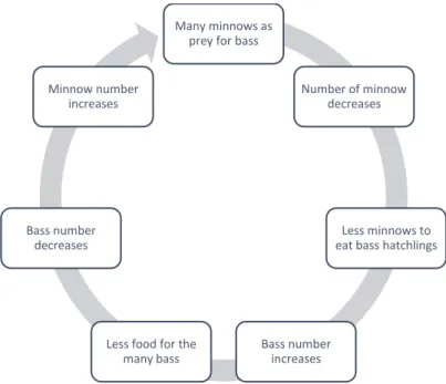
A typical example of critical slowing down is the ecosystem of a lake which changes to
another ecosystem when there are changing factors influencing the lake. The study by Carpenter
et al. (2011) describes the ecosystem of a lake in which there are two different types of fish: bass
and minnows. Both types of fish are predators and while the larger bass eat grown minnows,
those minnows prey on fleas but also bass hatchlings. Minnows are dominant in this system as
they decrease the number of bass that reach maturity and thus decrease the number of their
predator. The feedback loop of the ecosystem can be seen in Figure 1. This system is relatively
stable as the feedback loop pushes the ecosystem back into its stable equilibrium after a certain
time when it is only slightly perturbed (e.g. by adding a few more bass into the lake or by
Figure 1. Ecosystem feedback loop of a lake.
Larger changes such as a strong externally induced increase of bass population cannot be
equalized by the ecosystem as easily. In the experiment by Carpenter et al. (2011) a large number
of bass have been added to the already existing bass population to provoke a change in the
ecosystem. With an increase of the number of bass there is a decrease in minnow population as
they get preyed upon more and more. This leads to a further increase in bass population due to
the rising number of surviving bass hatchlings. Once the bass become the dominant predator, a
bass dominated lake is also relatively stable as a small increase of the number of minnows would
lead to increased prey for the bass which would therefore thrive, reducing the number of
minnows again.
Thus, there are two alternative stable states in this ecosystem, in the first one there are
many bass and few minnows. The other stable state is the original state before the experiment
with few bass and many minnows. In complex systems, as ecosystems or the human brain, a
simple feedback loop as in Figure 1 cannot describe all internal forces of the system, as many of
them are unknown, but might also support or prevent equilibration in an inaccessible way.
Therefore, the equilibration time after small perturbation might vary due to the internal state of
the system. An increase of the equilibration time after a small perturbation can be a warning sign
Many minnows as prey for bass
Number of minnow decreases
Less minnows to eat bass hatchlings
Bass number increases Less food for the
many bass Bass number
decreases Minnow number
for an upcoming change between stable states. When the equilibration slows down, former
perturbations might not have been equilibrated and cumulate over time, enforcing a transition.
During the transition between the stable states, there is no stability as the ecosystem is
changing from one state to the other. It is for instance not possible for an equal number of
minnows and bass to coexist in the lake over a longer period of time. During the period of
change, there are two alternative states that are ‘competing’ against each other, namely the
original state and the alternative state. When critically slowing down occurs the system will at
one point during the process switch from one feedback loop being the dominant one to the other
stable system being the dominant force. This point ‘of no return’ is called the tipping point of the
system.
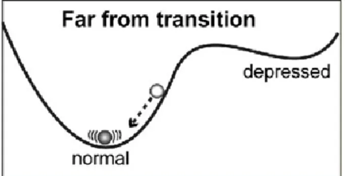
This phenomenon can be exemplified by the ball-in-the-cup phenomenon depicted in
Figure 2 and Figure 3. In a healthy individual or someone who is in remission, the state in which
it is easiest to get back to equilibrium is the normal state (Figure2). Even when disturbances are
major, the chance to fall into depression is much smaller than to revert to a normal state as it
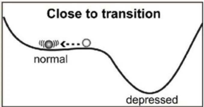
costs a lot of energy to do so. A change of the internal forces of a complex system like the human
brain might change this landscape. Once the tipping point is closer due to these changes it gets
more difficult to stay in the normal state (Figure 3). After small perturbances, it is likely to relax
to out of the stable normal state and into the alternative state. In this case, the alternative state is a
state of depression. The change from one state to the other is called the tipping point.
Figure 3. Ball-in-the-cup phenomenon in depression close to the transition (van de Leemput et al., 2014).
Wichers and Groot (2016) have shown that this critical slowing down before the tipping
point indeed happens in depression. During the time needed to relax back to equilibrium,
disturbances like stress can accumulate in the mental system. Mathematically, this slowing down
can be visible in increased variance and temporal autocorrelation (from one data point to the
next). The research by Wichers and Groot is mainly based on a previous study by Van de
Leemput et al. (2014) which had pioneered in this field of research by performing the first study
on critical slowing down in depression. Van de Leemput et al. set up a study in which the
participants assessed their emotions repeatedly during a period of several days. The participants
were healthy individuals as well as depressed patients. The findings showed that the
autocorrelations and variances were higher for participants who experienced a shift in depression
scores shortly after. This held true for depressed patients, who were about to experience
symptom worsening but also for those who were about to experience an improvement of their
symptoms.
Groot (2010), used ratings of physical activity additionally to mood ratings to assess his
depressive episode. The interaction between physical exercise and depression is a recent field of
research: Song, Lee, Baek, and Miller (2012) found an association of depression with a decreased
levels of exercise though it remained unsolved, whether this association is unidirectional. In a
recent meta-analysis, Mammen and Faulkner (2013) showed a preventive effect of regular
Our case has registered the number of times she did physical exercise in her diary from
the beginning, which made it possible for us to examine this variable. We will include her data on
the amount of physical exercise in our analysis to see, whether critical slowing down as a
warning sign for depression can be witnessed in the autocorrelation of the amount of exercise.
Next to mood symptoms and decreased physical activity, also decreased quality and
amount of sleep are typical for a depressive episode (Benca, Obermeyer, Thisted, & Gillin,
1992). Some literature even suggests that depression is partially maintained by insomnia
(Dombrovski et al., 2008). Moreover, several studies have shown that insomnia hinders recovery
and perpetuates depression in those suffering from both depression and insomnia (Kennedy,
Kelman, & Thomas, 1991; Pigeon et al., 2008). Thus, considering sleep as an additional variable
by including sleep ratings is necessary to paint a complete picture of a depressive episode.
The focus of this thesis will be to test the theory of critical slowing down in depression.
We will include several variables to represent different mood states, as well as exercise and sleep
ratings, to assess whether these factors show an enhanced autocorrelation directly before the
onset of depressive episodes. We expect autocorrelation to rise before the onset of the depressive
symptoms in all of the measurements.
Methods
Description of the case
The participant in this case study is a female born in 1964 and will be named Mrs. K. in
this paper. She is married and has two children, which were born in 1991 and 1993. Mrs. K.
suffered from recurrent depressive episodes throughout her life which she partially recorded in a
diary with eight different ratings. This diary is the basis for our analysis in which we analyzed
two different time spans regarding the appearance of critical slowing down within the data. The
diary contains daily ratings of mood, sleep, relaxation and trembling as well as records of the
menstrual cycle and exercise types. For this case study, we chose to concentrate on sleep,
exercise, relaxation and the different mood ratings.
In this paper we present the analysis of data from the diary written by the case at the time
before and during depressive episodes. We selected two time spans during which I know that a
depressive episode began. The case provided us with details on when she had recognized the
appearance of the depressive symptoms. According to the case, the starting point of the
symptoms, was in November in both episodes considered herein. We intended to include some
time before the starting point, as well as several weeks after, which led to an analysis of data
between the 15th September until the 31st December of the years 1997 and 2001. The period of analysis of the data before the depressive episode ranged from 15th September to 31st October. For the first episode, the subject had stated that the symptoms had appeared rather suddenly on
the 11th November. For the second episode, it was harder for the subject to point out a clear starting point. Nevertheless, she was certain that the depressive episode had also started in
November. This led to an observation window around the starting point for both episodes from
the 1st to the 31st November. The observation window of the time after the beginning of the depressive symptoms continued for the month of December. We decided to close the observation
window on the 31st December as we were interested in an increasing autocorrelation shortly before the beginning of a depressive episode only.
Instruments
The depression chapter of the English version of the M.I.N.I. 6.0 (Sheehan et al., 1998)
allows to assess symptoms and their severity of a depressive episode. We used this test to
evaluate Mrs. K.'s current status. Then we used this test to acquire information about the two
depressive episodes considered herein.
From all data that are protocolled by the case, we select six features for our analyses:
relaxation (‘Ontspanning’), physical exercise (‘Sport’), sleep (‘Slaap’), feelings (‘Gevoelen’), positive cognitions (‘Positive’) and activities during the day (‘Gedaan’). The three latter ones all
give indications on the mood of Mrs. K and will be combined later on.
In those scales Mrs. K used the following rating system: the variables ‘Gevoelen’,
‘Positive’ and ‘Gedaan’ had been protocolled by our case in a system equal to Dutch school
most negative. The variable ‘Ontspanning’ was classified on 3 occasions per day on a 3-point scale with the ratings ‘yes’, ‘yes/no’ and ‘no’. For the feature ‘Sport’, Mrs. K listed her activities
per day. The variable ‘Slaap’ was assessed on a scale using the categories positive, neutral and
negative sleep quality. Moreover, there were daily indications of whether the sleep was short or
restless.
Data preparation
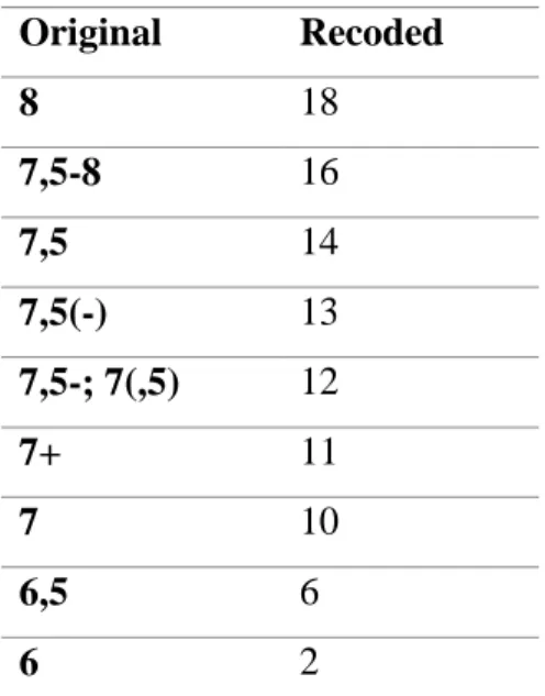
The original ratings of the mood variables consisted of a very limited range of ratings.
Even though the case had designed a rating from 1 to 10, the ratings varied between 7 and 8
mostly, with several intermediate ratings between those two numbers. After verifying the
meanings of those intermediary ratings with the case, we recoded them to prepare them for
analysis. In Table 1, one can find the original values, as well as the recoded values.
The variables sleep and relaxation were converted to a numerical three-point scale of 1
(negative), 2 (neutral) and 3 (positive). To assess overall sleep quality, shortness of sleep and
restlessness of sleep were dichotomously assessed (1 equals item is present, 0 equals item is not
present) included in a combined sleep variable. This variable was computed by the formula
2*sleep – (shortness + restlessness), which led to a scale between 0 and 6. We combined the three
ratings per day of the variable ‘Ontspanning’ into one daily rating by summing all three
classifications per this day. This led to a scale of 3 to 9. The daily sport variable was quantified
by counting the different sport activities at this day.
For further inspection, we also calculated a simple averaged autocorrelation of all
Original Recoded
8 18
7,5-8 16
7,5 14
7,5(-) 13
7,5-; 7(,5) 12
7+ 11
7 10
6,5 6
6 2
Table 1. Original and recoded values of the mood variables.
During our analyses we first used a change point analyzer on each episode to look out for
change points in the data which are not apparent by visual inspection. We then computed the
autocorrelation for each of the variables to look for a change that indicates critical slowing down
as a warning sign for the upcoming depressive episode. Before the change point analysis, we
used the ‘last observation carried forward’-principle to deal with missing data. This means, that if
any data is missing, the last known rating will be assumed for all the following missing ratings.
Statistical analysis
The analysis of change points included changes in each the mean and the variation in the
dataset using cumulative sum charts (CUSUM) and bootstrapping. CUSUM is a method that
calculates a cumulative sum Si, i being the number of observation. It does so by using the
difference between the average of all data X̅ and the value of each data point Xi and adding it to
the sum of the previous data point Si-1. The formula for this would be Si = Si-1 + (Xi - X̅) (Taylor, 2000). A bootstrapped CUSUM analysis is then used to find the confidence of the change visible
in the plot of the original CUSUM results. Bootstrapping is a procedure which includes
reordering the original values in a random order multiple times to see whether there is a true
change in the data. Change points can be found by looking at points with the biggest difference
then calculated by comparing the number of data points where the difference between the
maximum and minimum values is bigger in the original sample than in the bootstrapped sample.
Temporal autocorrelation r is the correlation of one observation with the previous observation and can be calculated via r = [∑𝑡=1𝑛 (Yt− Ȳ)(Yt+1− Ȳ)]/[∑𝑡= 1𝑛 (𝑌t− Ȳ)2]. Here, Ȳ denotes a
moving average using a 30-day window and t denotes the point of observation. Our data was investigated using visual inspection of the absolute temporal autocorrelation over time.
Results
First, we analyzed the results of the M.I.N.I. structured interview. This interview showed
that the case experienced several depressive episodes throughout her life. In total she lived
through seven depressive episodes. This provides evidence for the diagnosis of a major
depressive disorder in remission. The data provide evidence for each of the episodes in 1997 and
2001 which we will analyze in this paper. As depressive symptoms the case described consistent
negative mood, loss of interest and pleasure, decreased appetite, sleeping issues, restlessness and
difficulty concentrating. She continued to work during those episodes but her private life was
impaired due to the depression. Her first episode of depression began in 1980.
We then analyzed the two episodes of 1997 and 2001 individually regarding the change
point analyses and autocorrelation.
First Episode (1997)
According to the case, the symptoms of the first episode under consideration began
suddenly on November 11. The analysis window ranged from September 15, 1997 to December
31, 1997. In this time frame we found no significant change points in the data when using the
change point analysis. This may be reflecting the low variation in the data during that episode.
Our next step in analyzing the data was to inspect the autocorrelation as a possible
indication that critical slowing down exists as a precursor of a depressive episode. We used a
30-day moving window to calculate the autocorrelation for each of the variables (Feelings during the
day, positive cognitions, activity level, relaxation, exercise and sleep). We also calculated a mean
autocorrelation from those data. We inspected the individual figures of autocorrelation over time
each variable regarding a change in autocorrelation close to the presumed starting point of the
depression on November 11.
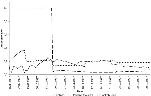
In Figures 4 through 7 one can find graphs of the temporal autocorrelation of the various
variables. As can be seen in Figure 4, a change in autocorrelation is clearly visible in regard to
the variable ‘Positive’. Namely, there is a sudden change of autocorrelation on the 18th October 1997 in which the autocorrelation decreases from 1 to 0.03. There is no other major change in
autocorrelation in this variable. The other two mood variables show less obvious changes in
autocorrelation. Nevertheless, closely around this date, there is also a subtler decrease visible on
the variable ‘Gedaan’ (from a value of 0.22 on October 17 to 0.13 on October 19). The
autocorrelation of this variable increases on the day, at which the case had recognized the
symptoms (November 11). From this date to the next day, there is an increase of 0.09. On the
variable ‘Gevoelen’, there is no major change of autocorrelation on these dates. There is an
increase in autocorrelation of this variable between the September 26 and the October 14. The
autocorrelation rises from 0.02 to 0.26 during this time. After that date, the autocorrelation of
‘Gevoelen’ decreases.
Figure 4. Autocorrelation of the three mood variables over time.
0,0 0,2 0,4 0,6 0,8 1,0 1 5 .0 9 .1 9 9 7 2 2 .0 9 .1 9 9 7 2 9 .0 9 .1 9 9 7 0 6 .1 0 .1 9 9 7 1 3 .1 0 .1 9 9 7 2 0 .1 0 .1 9 9 7 2 7 .1 0 .1 9 9 7 0 3 .1 1 .1 9 9 7 1 0 .1 1 .1 9 9 7 1 7 .1 1 .1 9 9 7 2 4 .1 1 .1 9 9 7 0 1 .1 2 .1 9 9 7 0 8 .1 2 .1 9 9 7 1 5 .1 2 .1 9 9 7 2 2 .1 2 .1 9 9 7 2 9 .1 2 .1 9 9 7 A u to c o rr e la ti o n Date
The autocorrelation of sleep and physical exercise is visible in Figure 5. In the variable
‘’Sport’ there is an increase of autocorrelation visible between September 25 and October 3.
After this date autocorrelation decreases. One can see a peak in autocorrelation on the day of the
presumed beginning of the depression, November 11 on the variable measuring the amount of
physical exercise (from 0.21 on November 10 to 0.25 on November 12). After this date, the
autocorrelation continues to decrease. On the variable ‘Sleep’ there are rather big changes in the
autocorrelation in the first two weeks of our measurement period and after this time span, the
autocorrelation tends to decrease. Around the presumed starting point of the depressive episode,
November 11, there is a decrease of autocorrelation of this variable visible. Namely, from
November 9 to November 11, autocorrelation decreases by 0.05. After this date, autocorrelation
increases. The autocorrelation of relaxation can be seen in Figure 6. There is an increase of
autocorrelation between September 26 and October 6. One can also see a major decrease of
autocorrelation shortly before the presumed starting date of the episode (from 0.25 on November
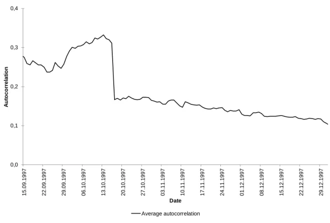
7 to 0.1 on November 12). In Figure 7, the average temporal autocorrelation of all previously
mentioned variables is presented. Autocorrelation increases until October 13. After that date, a
steep descend of autocorrelation can be observed (from 0.33 to 0.17 within four days). The
autocorrelation descends less steep after that point in time.
0,0 0,1 0,2 0,3 0,4 1 5 .0 9 .1 9 9 7 2 2 .0 9 .1 9 9 7 2 9 .0 9 .1 9 9 7 0 6 .1 0 .1 9 9 7 1 3 .1 0 .1 9 9 7 2 0 .1 0 .1 9 9 7 2 7 .1 0 .1 9 9 7 0 3 .1 1 .1 9 9 7 1 0 .1 1 .1 9 9 7 1 7 .1 1 .1 9 9 7 2 4 .1 1 .1 9 9 7 0 1 .1 2 .1 9 9 7 0 8 .1 2 .1 9 9 7 1 5 .1 2 .1 9 9 7 2 2 .1 2 .1 9 9 7 2 9 .1 2 .1 9 9 7 A u to c o rr e la ti o n Date Sleep Sport
Figure 5. Autocorrelation of sleep quality and physical exercise over time
In general, no clear trend or common change point is visible in the data. There is some
change in autocorrelation visible in the last 2 weeks of September and the first week of October.
This change does not give a clear indication of critical slowing down in this dataset. There are
also increasing and decreasing values of autocorrelation closely around the presumed starting
point of the depressive symptoms but there is no clear indication of critical slowing down either.
Figure 7. Average autocorrelation of the three mood variables, relaxation, exercise and sleep during the first episode.
Second Episode (2001)
The second depressive episode we investigated started, according to Mrs. K., in
November 2001. We again chose a time span from September 15 to December 31 to analyze this
episode. During this time there was no change in the variables ‘Positive’ and ‘Gedaan’. Those
variables were excluded in the analyses. The change point analysis yielded one change point
during this time span. The change point is situated on November 19, 2001 with a confidence
interval from September 26 to December 17. The level of confidence that the change point is
situated within this confidence interval is equal to 98%. Following, we will again evaluate
general trends in each of the variable. Furthermore, we will visually inspect the change point and
its confidence interval.
The autocorrelation of the mood variable ‘Gevoelen’ is shown in Figure 8. One can see a
general decline in autocorrelation over time. During the first two weeks of November, there is a
strong decrease in autocorrelation (from 0.36 to 0.19), followed by a strong increase during the
following two days (from 0.19 to 0.26). During the last week of November, where the change
point is situated, there is a decrease in autocorrelation by 0.07 during one day (November 26).
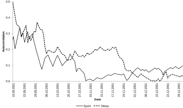
In Figure9, the autocorrelation of sleep and physical exercise is presented. In both, sleep
and sports, there is a downward trend visible in the first few weeks of the measurement period. In
the autocorrelation of physical exercise, this trend ends on October 31. After that date, the
autocorrelation rises again. One can see another decrease of autocorrelation around the presumed
change point. If one looks at the autocorrelation of sleep, it starts to increase around October 20
Figure 8. Autocorrelation of the mood variable over time during the second episode. 0,0 0,1 0,2 0,3 0,4 0,5 1 5 .0 9 .2 0 0 1 2 2 .0 9 .2 0 0 1 2 9 .0 9 .2 0 0 1 0 6 .1 0 .2 0 0 1 1 3 .1 0 .2 0 0 1 2 0 .1 0 .2 0 0 1 2 7 .1 0 .2 0 0 1 0 3 .1 1 .2 0 0 1 1 0 .1 1 .2 0 0 1 1 7 .1 1 .2 0 0 1 2 4 .1 1 .2 0 0 1 0 1 .1 2 .2 0 0 1 0 8 .1 2 .2 0 0 1 1 5 .1 2 .2 0 0 1 2 2 .1 2 .2 0 0 1 2 9 .1 2 .2 0 0 1 A u to c o rr e la ti o n Date Feelings 0,0 0,1 0,2 0,3 0,4 0,5 1 5 .0 9 .2 0 0 1 2 2 .0 9 .2 0 0 1 2 9 .0 9 .2 0 0 1 0 6 .1 0 .2 0 0 1 1 3 .1 0 .2 0 0 1 2 0 .1 0 .2 0 0 1 2 7 .1 0 .2 0 0 1 0 3 .1 1 .2 0 0 1 1 0 .1 1 .2 0 0 1 1 7 .1 1 .2 0 0 1 2 4 .1 1 .2 0 0 1 0 1 .1 2 .2 0 0 1 0 8 .1 2 .2 0 0 1 1 5 .1 2 .2 0 0 1 2 2 .1 2 .2 0 0 1 2 9 .1 2 .2 0 0 1 A u to c o rr e la ti o n Date Sport Sleep
The autocorrelation of relaxation can be seen in Figure10. There is no clear trend visible
in the data. There is a peak in autocorrelation in the middle of October (nearly 0.1), after that
peak, the autocorrelation varies between 0 and 0.05 with no major pattern visible. During the
time around the presumed change pint, there is a peak of 0.04 on November 24, followed by a
decrease until it reaches an autocorrelation of 0.
Figure 11 depicts the average autocorrelation of the mood variable, sports, sleep and
relaxation. There is a steady but slow decrease visible in autocorrelation during the whole
episode. No major change is visible around the change point.
Summary
All in all, in most of the variables, the autocorrelation does not clearly increase shortly
before the beginning of the depressive episodes. On the contrary, in some of the variables,
0,0 0,1 0,2 1 5 .0 9 .2 0 0 1 2 2 .0 9 .2 0 0 1 2 9 .0 9 .2 0 0 1 0 6 .1 0 .2 0 0 1 1 3 .1 0 .2 0 0 1 2 0 .1 0 .2 0 0 1 2 7 .1 0 .2 0 0 1 0 3 .1 1 .2 0 0 1 1 0 .1 1 .2 0 0 1 1 7 .1 1 .2 0 0 1 2 4 .1 1 .2 0 0 1 0 1 .1 2 .2 0 0 1 0 8 .1 2 .2 0 0 1 1 5 .1 2 .2 0 0 1 2 2 .1 2 .2 0 0 1 2 9 .1 2 .2 0 0 1 A u to c o rr e la ti o n Date Relaxation
autocorrelation seems to decrease around the beginning of the episode or the calculated change
point. Some of the variables could not be investigated in the second episode as they did not
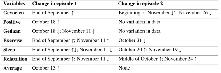
provide any variability. A summary of the results can be seen in Table 2. One can see that during
the first episode, a change in autocorrelation is visible in most variables in the end of September
and on the November 11, when the episode is presumed to have started. In episode 2 there is a
more diverse field of change points but almost all of them are situated in the end of November.
Variables Change in episode 1 Change in episode 2
Gevoelen End of September ↑ Beginning of November ↓↑; November 26 ↓
Positive October 18 ↑ No variation in data
Gedaan October 18 ↓; November 11 ↑ No variation in data
Exercise End of September ↑; November 11 ↑ October 31 ↓
Sleep End of September ↑↓; November 11 ↓ October 20 ↑; November 19 ↓
Relaxation End of September ↑; November 11 ↓ Middle of October ↑; November 24 ↑
Average October 13 ↑ None
Table 2. Summary of change points visible in the variables during the two episodes. ↓ depicting a decrease in autocorrelation; ↑ depicting an increase in autocorrelation
Discussion
We tested the hypothesis that autocorrelations of mood, sleep, relaxation and exercise
data rise shortly before the beginning of a depressive episode. Our analyses do not fully support
this hypothesis as autocorrelation did not increase directly before the beginning of a depressive
episode in all of the variables. During the first episode, there was an increase visible in all of the
three mood variables though all of those increases were on different dates, in different months
even. Only ‘Gedaan’, the record of the cases behavioral activities, shows an increase of
autocorrelation on November 11. Moreover, autocorrelation of sleep, exercise and relaxation
changes directly on the day that the symptoms were first apparent but only in ‘Sport’ the change
is visible as an increase of autocorrelation. In the second episode most relevant changes appear to
have happened in the end of November, which fits the results of the change point analysis as we
There is no clear pattern visible in autocorrelation, which indicates that there is not
enough supporting evidence for critical slowing down in this data. Previous research has been
able to indeed pinpoint increased autocorrelation as a possible precursor of a depressive episode
(van de Leemput et al., 2014; Wichers & Groot, 2016). As this field is not extensively researched
yet, there is not much evidence for critical slowing down in depression.
Bos and De Jonge (2014) have criticized Van de Leemput et al. (2014) for their research
methods in their letter. They suggest that Van de Leemput et al. (2014) claim a change in
individual scores, while the design only allows a comparison between subjects. Thus, the signs
for critical slowing down in those who developed a depressive episode later on may have been
due to higher baseline measures of those signs, instead of critical slowing down as a process
within a patient. Bos and De Jonge (2014) also stated that critical slowing down in general is not
to be overlooked. They rather suggested that there is more longitudinal within-subjects research
needed for the validation of the theory.
The fact that our research has not been able to provide evidence for the theory of critical
slowing down in depression may be due to the limitations of our study. One major limitation that
may have influenced this is the limited amount of data taken into account. As we analyzed only
one measurement per variable per day, there was a much lower number of total measurement
instances in our sample. This may have influenced the explanatory value of our analyses as the
autocorrelation may have varied much more from morning to afternoon, than it did from one day
to the next for instance. There may have been an increase in autocorrelation visible in subtler
changes during the day. Moreover, several measurement instances per day decreases the
probability of ‘noise’ influencing the ratings (e.g. time of the rating). Wichers and Groot (2016)
circumvented this issue by sampling data from the participant multiple times a day, which led to
more data in general and therefore more confidence in drawing conclusions. This was possible by
using technology to sample mood several times per day.
The possibilities of sampling using electronical devices have become more important
during the past decade. Through smartphone apps, electronical timing of the observation could
add validity to the observation as the subjects do not choose the time of measurement themselves
subjects’ mood that is closer to the natural diversity of mood during the day. Furthermore,
entering data electronically leads to the previous entry not being visible anymore. This adds value
to the rating as it is less dependent on the previous rating. This could provide an opportunity for
more sophisticated research on momentary emotional states. This has been used in the study by
Van de Leemput et al. (2014) for example. An extensive replication of this study would be
needed to provide more evidence for critical slowing down in depression.
One reason that could explain the absence of the tipping point might be found in the
partially missing data. In detail, 3 time-intervals with durations between 1 and 3 days of data
were missing and were filled by the ‘last observation carried forward’(LOCF)-principle. This
principle is widely used to handle dropouts and missing data as it is straightforward and provides
a first approximation for the missing data. Nevertheless, any retroactive filling of missing data
will inevitably introduce statistical errors. Therefore, the choice of appropriate filling methods is
under ongoing debate and also the drawbacks of the LOCF-principle are controversially
discussed in the literature (Overall, Tonidandel, & Starbuck, 2009; Saha & Jones, 2009). Errors
due to the retroactive complementation of the data will be more likely with the increasing
duration of the missing time intervals and could obscure the results.
In our dataset, there have been data with very little or no variation in the mood and
relaxation ratings. This may depict a truly small variation in the mental states of the participant
but it is also possible that this is due to the daily rating. As there is only one rating per day, the
subject may have averaged her mood over the day for the rating and this may have led to the flat
values. Furthermore, the rating scale was wide (1 to 10) but there was only a narrow window of
ratings used (6 to 9). There may be less variability due to the narrow rating use which leads to
less probability to find a change in autocorrelation. Although we tried to account for this when
changing the rating scale (see Table 1), this attempt might have been not sufficient enough
Moreover, the subject may have been influenced by the previous ratings as they were visible
when she rated the current day. This could have led to a less varying rating as she could have
feared to distance from the ‘normal’ rating.
The fact that this study has been analyzed as a case study brings positive, as well as
no possibility to generalize to any population as there is only one subject in our study and all of
the results may be due to the properties of this case.
Furthermore, the results may be completely unrelated to the depressive episodes. If one
looks at the bigger picture, there are many changes in the dataset and most of the changes we
have found are not on or even around the same date. This could indicate that the change may be
due to different factors which also show in the autocorrelation, such as seasonal components or
life events.
This paper did not find enough evidence for critical slowing down in physical exercise
and sleep. This may be due to flaws in our design but there is always the possibility that, even if
slowing down is a precursor of a depressive episode, sleep and exercise are not closely enough
related to depression to show the critical slowing down in detail. More research is needed which
includes sleep and physical exercise as possible factors showing critical slowing down in
depression.
Measuring symptoms on a daily basis seems to have brought benefit to both, our case and
Groot (2010), otherwise they would not have continued to record it over a long period of time.
Thus, there seems to be a beneficial value in recording mood, activity, sleep and other items
associated to depression. To investigate the effect of this form of self-therapy and its working
mechanism could be the focus of further research as well.
Using several cases or a larger trial in further studies could add significant value to this
field of research. Validity would increase by not using multiple individual. Suitable individuals
would be subjects who already had multiple episodes of depression and who are possible
candidates for further episodes in the future. Monitoring them over several years could give
insights on how depressive episodes approach and whether there is critical slowing down in
depression.
Although this investigation did not provide strongly conclusive results, it still enhanced
the knowledge of the research field by providing a new direction for research, including exercise
and sleep as possible factors. There is still a wide variety of possibilities for further research,
Appendix 1
Figure 1. Ecosystem feedback loop of a lake.
Many minnows as prey for bass
Number of minnow decreases
Less minnows to eat bass hatchlings
Bass number increases Less food for the
many bass Bass number
decreases
Appendix 2
Appendix 3
Appendix 4
Figure 4. Autocorrelation of the three mood variables over time during the first episode.
0,0 0,2 0,4 0,6 0,8 1,0 1 5 .0 9 .1 9 9 7 2 2 .0 9 .1 9 9 7 2 9 .0 9 .1 9 9 7 0 6 .1 0 .1 9 9 7 1 3 .1 0 .1 9 9 7 2 0 .1 0 .1 9 9 7 2 7 .1 0 .1 9 9 7 0 3 .1 1 .1 9 9 7 1 0 .1 1 .1 9 9 7 1 7 .1 1 .1 9 9 7 2 4 .1 1 .1 9 9 7 0 1 .1 2 .1 9 9 7 0 8 .1 2 .1 9 9 7 1 5 .1 2 .1 9 9 7 2 2 .1 2 .1 9 9 7 2 9 .1 2 .1 9 9 7 A u to c o rr e la ti o n Date
Appendix 5 0,0 0,1 0,2 0,3 0,4 1 5 .0 9 .1 9 9 7 2 2 .0 9 .1 9 9 7 2 9 .0 9 .1 9 9 7 0 6 .1 0 .1 9 9 7 1 3 .1 0 .1 9 9 7 2 0 .1 0 .1 9 9 7 2 7 .1 0 .1 9 9 7 0 3 .1 1 .1 9 9 7 1 0 .1 1 .1 9 9 7 1 7 .1 1 .1 9 9 7 2 4 .1 1 .1 9 9 7 0 1 .1 2 .1 9 9 7 0 8 .1 2 .1 9 9 7 1 5 .1 2 .1 9 9 7 2 2 .1 2 .1 9 9 7 2 9 .1 2 .1 9 9 7 A u to c o rr e la ti o n Date Sleep Sport
Appendix 6 0,0 0,1 0,2 0,3 0,4 1 5 .0 9 .1 9 9 7 2 2 .0 9 .1 9 9 7 2 9 .0 9 .1 9 9 7 0 6 .1 0 .1 9 9 7 1 3 .1 0 .1 9 9 7 2 0 .1 0 .1 9 9 7 2 7 .1 0 .1 9 9 7 0 3 .1 1 .1 9 9 7 1 0 .1 1 .1 9 9 7 1 7 .1 1 .1 9 9 7 2 4 .1 1 .1 9 9 7 0 1 .1 2 .1 9 9 7 0 8 .1 2 .1 9 9 7 1 5 .1 2 .1 9 9 7 2 2 .1 2 .1 9 9 7 2 9 .1 2 .1 9 9 7 A u to re g re s s io n Date Relaxation
Appendix 7 0,0 0,1 0,2 0,3 0,4 1 5 .0 9 .1 9 9 7 2 2 .0 9 .1 9 9 7 2 9 .0 9 .1 9 9 7 0 6 .1 0 .1 9 9 7 1 3 .1 0 .1 9 9 7 2 0 .1 0 .1 9 9 7 2 7 .1 0 .1 9 9 7 0 3 .1 1 .1 9 9 7 1 0 .1 1 .1 9 9 7 1 7 .1 1 .1 9 9 7 2 4 .1 1 .1 9 9 7 0 1 .1 2 .1 9 9 7 0 8 .1 2 .1 9 9 7 1 5 .1 2 .1 9 9 7 2 2 .1 2 .1 9 9 7 2 9 .1 2 .1 9 9 7 A u to re g re s s io n Date Average autoregression
Figure 7. Average autocorrelation of the three mood variables, relaxation, exercise and
Appendix 8
Figure 8. Autocorrelation of the mood variable over time during the second episode.
Appendix 9 0,0 0,1 0,2 0,3 0,4 0,5 1 5 .0 9 .2 0 0 1 2 2 .0 9 .2 0 0 1 2 9 .0 9 .2 0 0 1 0 6 .1 0 .2 0 0 1 1 3 .1 0 .2 0 0 1 2 0 .1 0 .2 0 0 1 2 7 .1 0 .2 0 0 1 0 3 .1 1 .2 0 0 1 1 0 .1 1 .2 0 0 1 1 7 .1 1 .2 0 0 1 2 4 .1 1 .2 0 0 1 0 1 .1 2 .2 0 0 1 0 8 .1 2 .2 0 0 1 1 5 .1 2 .2 0 0 1 2 2 .1 2 .2 0 0 1 2 9 .1 2 .2 0 0 1 A u to c o rr e la ti o n Date Sport Sleep
Appendix 10 0,0 0,1 0,2 1 5 .0 9 .2 0 0 1 2 2 .0 9 .2 0 0 1 2 9 .0 9 .2 0 0 1 0 6 .1 0 .2 0 0 1 1 3 .1 0 .2 0 0 1 2 0 .1 0 .2 0 0 1 2 7 .1 0 .2 0 0 1 0 3 .1 1 .2 0 0 1 1 0 .1 1 .2 0 0 1 1 7 .1 1 .2 0 0 1 2 4 .1 1 .2 0 0 1 0 1 .1 2 .2 0 0 1 0 8 .1 2 .2 0 0 1 1 5 .1 2 .2 0 0 1 2 2 .1 2 .2 0 0 1 2 9 .1 2 .2 0 0 1 A u to c o rr e la ti o n Date Relaxation
Appendix 11 0,0 0,1 0,2 0,3 0,4 0,5 1 5 .0 9 .2 0 0 1 2 2 .0 9 .2 0 0 1 2 9 .0 9 .2 0 0 1 0 6 .1 0 .2 0 0 1 1 3 .1 0 .2 0 0 1 2 0 .1 0 .2 0 0 1 2 7 .1 0 .2 0 0 1 0 3 .1 1 .2 0 0 1 1 0 .1 1 .2 0 0 1 1 7 .1 1 .2 0 0 1 2 4 .1 1 .2 0 0 1 0 1 .1 2 .2 0 0 1 0 8 .1 2 .2 0 0 1 1 5 .1 2 .2 0 0 1 2 2 .1 2 .2 0 0 1 2 9 .1 2 .2 0 0 1 A u to c o rr e la ti o n Date Average autocorrelation
Figure 11. Average autocorrelation of the mood variable, exercise, sleep and relaxation
Appendix 12
Original Recoded
8 18
7,5-8 16
7,5 14
7,5(-) 13
7,5-; 7(,5) 12
7+ 11
7 10
6,5 6
6 2
Appendix 13
Variables Change in episode 1 Change in episode 2
Gevoelen End of September ↑ Beginning of November ↓↑; November 26 ↓
Positive October 18 ↑ No variation in data
Gedaan October 18 ↓; November 11 ↑ No variation in data
Exercise End of September ↑; November 11 ↑ October 31 ↓
Sleep End of September ↑↓; November 11 ↓ October 20 ↑; November 19 ↓
Relaxation End of September ↑; November 11 ↓ Middle of October ↑; November 24 ↑
Average October 13 ↑ None
References
Benca, R. M., Obermeyer, W. H., Thisted, R. A., & Gillin, J. C. (1992). Sleep and Psychiatric
Disorders. Archives of General Psychiatry, 49(8), 651. http://doi.org/10.1001/archpsyc.1992.01820080059010
Bos, E. H., & De Jonge, P. (2014). “Critical slowing down in depression” is a great idea that still
needs empirical proof. Proceedings of the National Academy of Sciences of the United States of America, 111(10), E878. http://doi.org/10.1073/pnas.1323672111
Carpenter, S. R., Cole, J. J., Pace, M. L., Batt, R., Brock, W. a., Cline, T., … Weidel, B. (2011).
Early Warnings of Regime Shifts: A Whole-Ecosystem Experiment. Science, 332(6033), 1079–1082. http://doi.org/10.1126/science.1203672
Diamond, M., & Sigmundson, H. K. Sex reassignment at birth. Long-term review and clinical
implications., 151 Archives of pediatrics & adolescent medicine 298–304 (March 1997).
http://doi.org/10.1001/archpedi.1997.02170470096022
Dombrovski, A. Y., Cyranowski, J. M., Mulsant, B. H., Houck, P. R., Buysse, D. J., Andreescu,
C., … Frank, E. (2008). Which symptoms predict recurrence of depression in women treated
with maintenance interpersonal psychotherapy? Depression and Anxiety, 25(12), 1060–
1066. http://doi.org/10.1002/da.20467
Groot, P. C. (2010). Patients can diagnose too: How continuous self-assessment aids diagnosis of,
and recovery from, depression. Journal of Mental Health (Abingdon, England), 19(4), 352– 62. http://doi.org/10.3109/09638237.2010.494188
Harlow, J. M. (1848). Passage of an iron rod through the head. Boston Medical and Surgical Journal. http://doi.org/10.1056/NEJM184812130392001
Kazdin, A. E. (2014). Research Design in Clinical Psychology. Allyn and Bacon.
Kennedy, G. J., Kelman, H. R., & Thomas, C. (1991). Persistence and remission of depressive
http://ovidsp.ovid.com/ovidweb.cgi?T=JS&PAGE=reference&D=med3&NEWS=N&AN=1
824809
Mammen, G., & Faulkner, G. (2013). Physical Activity and the Prevention of Depression.
American Journal of Preventive Medicine, 45(5), 649–657. http://doi.org/10.1016/j.amepre.2013.08.001
Overall, J. E., Tonidandel, S., & Starbuck, R. R. (2009). Last-observation-carried-forward
(LOCF) and tests for difference in mean rates of change in controlled repeated
measurements designs with dropouts. Social Science Research, 38(2), 492–503. http://doi.org/10.1016/j.ssresearch.2009.01.004
Pigeon, W. R., Hegel, M., Unützer, J., Fan, M.-Y., Sateia, M. J., Lyness, J. M., … Perlis, M. L.
(2008). Is insomnia a perpetuating factor for late-life depression in the IMPACT cohort?
Sleep, 31(4), 481–488.
Saha, C., & Jones, M. P. (2009). Bias in the last observation carried forward method under
informative dropout. Journal of Statistical Planning and Inference, 139(2), 246–255. http://doi.org/10.1016/j.jspi.2008.04.017
Sheehan, D. V, Lecrubier, Y., Sheehan, K. H., Amorim, P., Janavs, J., Weiller, E., … Dunbar, G.
C. (1998). The Mini-International Neuropsychiatric Interview (M.I.N.I.): the development
and validation of a structured diagnostic psychiatric interview for DSM-IV and ICD-10. The Journal of Clinical Psychiatry, 59 Suppl 2, 22–33;quiz 34–57. Retrieved from
http://www.ncbi.nlm.nih.gov/pubmed/9881538
Skinner, B. F. (1938). Conditioning and Extinction. In R. M. Elliot (Ed.), The Behavior of
Organisms: An experimental analysis (pp. 61–115). Minneapolis, United States of America: D. Appleton-Century Company, Inc. http://doi.org/10.1037/h0052216
Song, M. R., Lee, Y.-S., Baek, J.-D., & Miller, M. (2012). Physical Activity Status in Adults with
Depression in the National Health and Nutrition Examination Survey, 2005-2006. Public Health Nursing, 29(3), 208–217. http://doi.org/10.1111/j.1525-1446.2011.00986.x
Retrieved August 3, 2016, from http://www.variation.com/cpa/tech/changepoint.html
Ter Kuile, M. M., Bulté, I., Weijenborg, P. T. M., Beekman, A., Melles, R., & Onghena, P.
(2009). Therapist-aided exposure for women with lifelong vaginismus: a replicated
single-case design. Journal of Consulting and Clinical Psychology, 77(1), 149–159. http://doi.org/10.1037/a0014273
van de Leemput, I. a, Wichers, M., Cramer, A. O. J., Borsboom, D., Tuerlinckx, F., Kuppens, P.,
… Scheffer, M. (2014). Critical slowing down as early warning for the onset and
termination of depression. Proceedings of the National Academy of Sciences of the United States of America, 111(1), 87–92. Retrieved from
http://www.pubmedcentral.nih.gov/articlerender.fcgi?artid=3890822&tool=pmcentrez&rend
ertype=abstract
Watson, J. B., & Rayner, R. (1920). Conditioned emotional reactions. Journal of Experimental Psychology, 3(1), 1–14. http://doi.org/10.1037/h0069608
Wichers, M., & Groot, P. C. (2016). Critical Slowing Down as a Personalized Early Warning
Signal for Depression. Psychotherapy and Psychosomatics, 85(2), 114–6.