EVALUATING CURRENT PRACTICES IN MEASURING AND MODELING ADOLESCENT ALCOHOL FREQUENCY DATA
James S. McGinley
A thesis submitted to the faculty of the University of North Carolina at Chapel Hill in partial fulfillment of the requirements for the degree of Master of Arts in the Department of
Psychology.
Chapel Hill 2011
ABSTRACT
JAMES S. MCGINLEY: Evaluating Current Practices in Measuring and Modeling Adolescent Alcohol Frequency Data
(Under the direction of Patrick Curran)
Substance use is a significant health risk behavior from both developmental and public health perspectives. In recent years, there has been substantial growth in the
theoretical conceptualization of pathways to substance use during adolescence. However, in order to test these developmental theories researchers must be able to validly measure and model substance use. This project evaluated the current standard practices in measuring and modeling adolescent alcohol frequency data. Using a simulation study and empirical
ACKNOWLEDGEMENTS
TABLE OF CONTENTS
LIST OF TABLES………..…….…………vi
LIST OF FIGURES………vii
I. CURRENT PRACTICES IN MEASURING AND MODELING ADOLESCENT ALCOHOL FREQUENCY DATA………...….1
II. METHOD………..………..17
III. RESULTS………...……….27
IV. DISCUSSION………..……….….………..36
LIST OF TABLES
Table
1. Table 1. Four alcohol frequency scales for a past 30 day time frame………...…...47 2. Table 2. Experimental seven point measure based on the log transformation……….48 3. Table 3. Recovery of population generating values from simulation…………...49 4. Table 4. Simulation Condition 1: Proportion of significant effects, Type I and II
Errors, ORs, and standardized regression coefficients………...…….50 5. Table 5. Simulation Condition 2: Proportion of significant effects, Type I and II
errors, ORs, and standardized regression coefficients……….………51 6. Table 6. Simulation Condition 3: Proportion of significant effects, Type I and II
Errors, ORs, and standardized regression coefficients……….…...52 7. Table 7. Simulation Condition 4: Proportion of significant effects, Type I and II
errors, ORs, and standardized regression coefficients………...53 8. Table 8. Simulation: Percent of different patterns effect caused by scoring across
measures………...54 9. Table 9. Simulation: Percent of different patterns effect caused by scale across
scoring approaches………...55 10.Table 10. Empirical Demonstration: Proportion of significant effects, OR compared
LIST OF FIGURES
Figure
1. Figure 1. Histograms for normal, negative binomial, and zero-inflated negative binomial distribution………....…..……….57 2. Figure 2. Histograms for ZINB counts and NIAAA ordinal scale…………..……...58 3. Figure 3. Simulation Study, Condition 1: Marginal distribution of counts……....…59 4. Figure 4. Empirical Demonstration: Marginal distribution of alcohol frequency
Evaluating Current Practices in Measuring and Modeling Adolescent Alcohol Frequency Data
Adolescent substance use is a widespread concern in the United States. The Monitoring the Future (MTF) study, a national school-based survey, found that in 2009, 36.6% of 8th graders, 59.1% of 10th graders, and 72.3% of 12th graders reported drinking alcohol at least once in their lifetime and 17.4% of 8th graders, 38.6% of 10th graders, and 56.5% of 12th graders reported getting drunk at least once in their lifetime (Johnston, O’Malley, Bachman, & Schulenberg, 2009). In 2001 alone, it was estimated that underage
drinking cost the United States 61 billion dollars (Miller, Levy, Spicer, & Taylor, 2006). More concerning are the non-monetary consequences of adolescent substance use. In the short-term, adolescent substance use is associated with morbidity, driving accidents, risky sexual behavior, and even death (USDHHS, 2007). There is also evidence that substance use in adolescence has negative long-term biological effects such as disruptions in
neuropsychological development and performance (Tapert, Caldwell, & Burke, 2005) and female pubertal development (Emanuele, Wezeman, & Emanuele, 2002). Several studies have found a relationship between adolescent substance use and lower educational attainment, difficulties transitioning from adolescence into young adulthood (Hussong & Chassin, 2002), and psychological problems in adulthood (Trim, Meehan, King, & Chassin, 2007). Clearly, adolescent substance use is a significant public health concern.
Maslowsky, 2009). Deviance proneness models, which operate off the tenet that substance use occurs along with the development of general conduct problems, and biological models, which posit that adolescents with family histories of drug abuse and dependence are at
greater risk for substance use, have been well supported by prior research (Chassin, Hussong, & Beltran, 2009; Chassin, Presson, Pitts, & Sherman, 2000). On the other hand, empirical tests of the relationship between internalizing symptomatology and the etiology of substance use in adolescence remain inconclusive with some studies reporting a significant association between them (Chassin, Pillow, Curran, Molina, & Barrera, 1993; Cooper, Frone, Russell, & Mudar, 1995), while others have failed to find such a link (Hallfors, Waller, Bauer, Ford, & Halpern, 2005; Hussong, Curran, & Chassin, 1998). This tremendous growth in adolescent substance use research over the past decade and a half needs to continue well into the future.
However, in order to empirically evaluate any of these theories, researchers must be able to validly and reliably measure and model the substance use outcomes of interest. Substance use measures examine alcohol or other drugs such as marijuana, cocaine, and heroin. Dimensions of substance use commonly examined include abuse, dependence, consequences, and frequency and quantity of use. It has been well documented that many adolescent substance use measures lack sufficient psychometric properties (Leccese & Waldron, 1994). In part, this psychometric deficiency is caused by the complex nature of adolescent substance use measurement. For instance, it is difficult to determine the reliability and validity of instruments that assess multiple substances (e.g., alcohol, cigarettes,
project focused strictly on frequency of alcohol use. The issues studied in this project are expected to generalize to other substances.
Measuring Alcohol Use
Over the past half-century, numerous alcohol use measures have been proposed, most of which can be classified into one of three categories: daily drinking, lifetime drinking, and quantity-frequency measures. First, daily drinking measures assess daily alcohol
consumption for a specified time period (e.g., Sobell and Sobell’s (2000) Alcohol Timeline Followback (TLFB) and Miller and Del Boca’s (1994) Form 90). Advantages of these
Researchers often choose to utilize either the quantity per drinking day or frequency of alcohol use independently to test specific research hypotheses. Quantity-frequency measures offer several practical advantages such as short administration time, easy computations, intuitive meaning, and researchers can use quantity or frequency measures separately to test unique effects involving alcohol use. However, these methods have been criticized on a variety of grounds including the underestimation of true alcohol consumption, as well as the omission of important information about variability in alcohol consumption patterns (Dawson & Room, 2000; Ivis, Bondy, & Adlaf, 1997; Sobell & Sobell, 1995).
In this project, I focused on frequency of alcohol use because it is widely used in applied research and the findings likely generalize to similar types of substance use
measures. By definition, alcohol frequency data are counts because participants report on the number of days in which they drank alcohol over a given timeframe. Despite this fact, most researchers provide binned ordinal response categories for frequency of alcohol use (e.g., 1-3 times a month, 1 time per week, etc.) rather than leaving responses open-ended because it lessens participant burden and errors in cognitive recall (Ivis et al., 1997). To help
standardize these measures, the National Council on Alcohol Abuse and Alcoholism
established and recommended sets of alcohol consumption questions, totaling between 3 and 6 questions (NIAAA, 2003). An example of a frequency item modified for a past 30 day timeframe is displayed in the first column of Table 1. Importantly, the committee
recommended using binned ordinal response categories.
investigating how these alcohol frequency measures perform when testing theories of adolescent alcohol use with misspecified statistical models (e.g., fitting linear models to ordinal data). Even if an alcohol measure has strong traditional psychometric support, it can still produce invalid tests of substantive theories in commonly used statistical models.
For example, consider if there was a true effect of age on frequency of alcohol use such that older adolescents, on average, drank more frequently than younger adolescents. Two researchers may measure frequency of alcohol in the same participants using two different measures; one with five point scales the other with a 12 point scale, assuming perfect reliability from the reporter. Although both of these measures show strong traditional psychometrics properties and the same statistical model is fitted to the data, one model may find a significant age effect while the other does not because of a reduction in statistical power moving from 12 categories to five categories (MacCallum, Zhang, Preacher, & Rucker, 2002; Taylor, West, & Aiken, 2006). For another example, assume alcohol
frequency is measured with two seven point scales with response categories characterized by different bin sizes. A model fitted to the data derived from one of the seven point scales could produce a significant age effect while the age effect turns out to be non-significant using the other seven point scale. This discrepancy has the potential to occur in practice because different binning methods may produce different relationships between a set of covariates and the outcome. These two inconsistences exemplify invalidity in testing
Current Practices in Modeling Alcohol Frequency Data
The standard practice in adolescent substance use research is to test theoretical models by treating an ordinal alcohol frequency outcome as continuous in a linear statistical method (A few recent examples of this are Dogan, Stockdale, Widaman, and Conger, 2010; Rice, Milburn, & Monro, 2011; Patrick & Schulenberg, 2011). These linear models are not ideal from a statistical standpoint, but researchers use this strategy because alternative statistical models are not well studied or readily available (Curran & Willoughby, 2003). Furthermore, closer examination of the distributional properties and generalized model techniques for discrete alcohol frequency data helps to clarify why standard linear models are so widely utilized by alcohol researchers. Through briefly exploring the Generalized Linear Model (GLM) framework, I will provide insights as to why using ordinal alcohol frequency data in traditional linear models can lead to invalid tests of substantive theory.
Distributions of Alcohol Frequency Data
Alcohol researchers frequently treat ordinal alcohol frequency data as continuous in linear models. In doing so, they inherently assume that the ordinal outcome follows the probability density function (pdf) for the normal distribution
(1)
2 1 ) ( 2 2 2 ) ( 2 y e y P
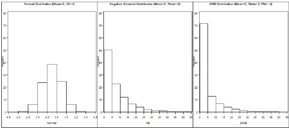
The parameters and 2are the mean and standard deviation. Figure 1 shows the standard
normal distribution with 0 and 2 1. This pdf shows that alcohol frequency cannot be
frequency counts are characterized by a large proportion of non-alcohol users, also known as zero-inflation in the statistics literature. For this reason, alcohol frequency counts likely conform to a negative binomial distribution rather than the more familiar Poisson distribution because its added dispersion parameter allows for much more flexibility. The probability mass function (pmf) for the negative binomial distribution can be expressed as
) 2 ( ,... 2 , 1 , 0 , ) )( ( ) 1 ( ) ( ) ( ) (
y
y y y P x g y y
where the distribution has mean of and a variance of (1(1/)). Figure 1 show the
negative binomial distribution with 2 and .8. A dual process, zero-inflated negative binomial (ZINB) process is a second viable option for characterizing adolescent alcohol frequency data. The ZINB probability function can be expressed as
(3)
0 ) ( ) 1 ( 0 ) 0 ( ) 1 ( ) ( y if y g y if g y P
where is the probability of zero counts and the function g(.) represents counts drawn from the negative binomial distribution as described in Eq. 2. Figure 1 shows the ZINB
distribution after adding an excess zero probability .42to negative binomial distribution described above. This probability function for the ZINB implies that zeros are generated from two sources: (1) the inflated zeros probability (e.g., structural zeros) and (2) the expected zeros from a negative binomial distribution (e.g., sampling zeros).
after binning the counts into ordinal categories based on NIAAA scale from Table 1. This binning process makes the selection and implementation of an appropriate statistical method for validly testing theoretical hypotheses of adolescent alcohol use challenging for applied research.
Clearly, there is a disconnect between the distributions associated with the underlying count of days using alcohol (Equations 2 and 3) and what researchers often assume in
statistical models (Equation 1). This incongruity is worsened by the process of binning frequency counts in ordinal categories. By briefly exploring the GLM, I will highlight why adolescent alcohol researchers often use linear models for ordinal alcohol frequency data and form the foundation for describing how linear models fit to ordinal data can lead to invalid statistical inferences.
Generalized Linear Model (GLM) and Alcohol Frequency Data
The GLM offers a unifying modeling framework that subsumes traditional continuous linear models with various models for discrete outcomes. The GLM operates on three
components: (1) Stochastic Component - this is commonly thought of as the error structure of response distribution, (2) Systematic Component - this is how the predictors affect the
outcome that is transformed through the specified link function (e.g., θXβ), and (3) Link
Function –this connects the Stochastic Component with the Systematic Component (e.g.
Xβ θ
μ)
(
g ). I will next lay out how the GLM encompasses continuous and discrete
outcomes.
) 4 (
Xβ
μ
where X is an n x p matrix of covariates,βis p x 1 vector of regression coefficients, and the
outcome follows a normal distribution (e.g., multiple regression, ANOVA). However, if researchers were fitting models to the underlying count of the number of data of alcohol use, they would likely use a logarithmic link function such that
log(μ)Xβ (5) where X is an n x p matrix of covariates,βis p x 1 vector of regression coefficients, and the
outcome follows a negative binomial distribution. The ZINB model may also be useful for modeling adolescent alcohol data. The ZINB model is a two-component mixture model combining a point mass at zero with a negative binomial distribution. Zeros arise from two sources, the probability of excess zeros and the zeros naturally occurring in the NB
distribution. The mean models for the ZINB model can be expressed as
μ0(1)exp(Xβ) (6)
where X is an n x p matrix of covariates,βis p x 1 vector of regression coefficients for the
count process, and the outcome follows a negative binomial distribution. The unobserved probability of excess zeros is modeled with a binomial GLM with a logit link as
logit()Zγ (7)
Z is an n x q matrix of covariates, is q x 1 vector of regression coefficients for the zero process, and the outcome follows a binomial distribution. Alcohol researchers rarely collect frequency data as open-ended counts, so we can consider a basic ordinal model: the
proportional odds model which is defined as
The outcome is now modeled as cumulative logits, which are simply logits of cumulative probabilities for the j response categories. Each cumulative logit has its own intercept
expressed as jand the model implies the same effect,β, for each logit (this is the
“proportional odds” assumption). The outcome is assumed to follow a multinomial
distribution. These models are quite complex and have strong assumptions, which are often unfeasible for alcohol frequency data. For instance, a frequency scale with 10 response categories would need to have 9 intercepts. This is precisely why applied researchers fit linear models such as described in Equation 4 to ordinal alcohol frequency data.
There are stark differences between the models expressed in Equations 4 through 8. Fitting the negative binomial model is often not an option because alcohol frequency counts are seldom collected by researchers. Although the utilization of linear statistical models to ordinal alcohol frequency data is often defensible from a practicality standpoint, these models are highly susceptible to producing invalid statistical inferences. The factors producing these invalid inferences can again be tied to the GLM framework.
Alcohol Frequency and Validity of Inferences
approaches: category numbers and the midpoint value within each ordinal category. In practice, both of these factors vary in adolescent alcohol use applications and there is currently no gold standard alcohol frequency measure or scoring approach. Often times, researchers do not even report the characteristics of a measure or how they scored the ordinal alcohol variable. In my project, I will empirically examine whether or not these two factors are critical for validly testing theories of adolescent alcohol use.
Characteristics of Alcohol Frequency Measures
The quantitative elements of alcohol frequency measures are the number of ordinal response categories and the method of binning the underlying days of alcohol use counts into ordinal response categories. While prior quantitative research suggests that a larger number of response categories should be better suited for testing models of adolescent alcohol use than fewer categories because researchers lose less information (Taylor, West, & Aiken, 2006), it is unclear how the method of binning underlying counts into ordinal categories affects statistical inferences. It is plausible that the number of categories may interact with binning strategies such that the effect of the number of ordinal categories on the validity of results generated from statistical models depends on how the response categories are binned.
Quantitative researchers refer to the process of binning an underlying continuous or count quantitative variable into a smaller number of ordered categories as coarse
categorization (Taylor, West, & Aiken, 2006). Several studies have shown that coarse categorization can be problematic from a quantitative standpoint. For instance, MacCallum, Zhang, Preacher, and Rucker (2002) detailed the statistical repercussions caused by
West, and Aiken (2006) expanded this work to show that coarsely categorized ordinal outcomes lead to a loss of power in logistic, ordinal logistic, and probit regression. Findings from this study suggest that, typically, more categories that have a rectangular distribution are better than fewer categories that are skewed. However, this study assumed that
underlying these categories was a normal continuous variable.
Far less information exists about the statistical implications of binning counts into a series of unequally spaced ordinal responses, which is the case for alcohol frequency measures. Note that for the NIAAA alcohol frequency question, moving from the zero category to the one category is not the same as moving from the three category to the four category. As previously stated, alcohol researchers use ordinal measures with unequal categories to minimize errors in cognitive recall. However, the implications of using these measures with standard linear models are currently unclear. It appears that binning alcohol frequency counts into categories may act as pseudo data transformation. Consider the popular logarithmic transformation for use in linear models, which converts multiplicative
Equation 5 displays the negative binomial model. Notice that the appropriate
nonlinear link function is the logarithmic link. The regression coefficients can be interpreted in terms of changes in the transformed mean response in the study population, and their relation to the set of covariates. From a statistical standpoint, it appears that a strategy that bins alcohol frequency counts in increasingly larger categories that mirror the logarithmic transformation should be best for linear modeling (assuming one uses the category number as the alcohol frequency scores). However, in practice, there is no widely accepted method for defining alcohol frequency categories. Most researchers do not report the response scales of their alcohol frequency measures in academic journals so the extent to which measures vary in practice is unknown. Prior research in statistics has shown that applying different data transformations to the same data can indeed lead to different patterns of statistical
significance and inaccurate predictions (Adams, 1991; O’Hara & Kotze, 2010). Extending
this finding to adolescent alcohol use, it is expected that the more these alcohol measures vary in their binning approaches (e.g., the more the pseudo data transformations differ), the more likely researchers are to observe invalid patterns of effects caused solely by
measurement.
Scoring Approaches for Alcohol Frequency Data
frequency measure, the scores would be 0, 1, 2.5, 4.5, 7.5, and so on. Although the
differences between these scoring methods appear trivial, they have the ability to seriously impact the validity of hypothesis tests concerning adolescent alcohol use. These scoring approaches for ordinal data have yet to be systematically studied in the context of adolescent alcohol use.
From a statistical viewpoint, the category number scoring approach appears advantageous to the median approach. As previously described, many ordinal alcohol frequency measures functionally work as a data transformation that helps to linearize the relationship between a set of predictors and the alcohol frequency outcome. This is consistent with the logarithmic link model expressed in Equation 5. Conversely, the median approach takes the ordinal alcohol frequency response and converts it back to a metric similar to the underlying frequency count (e.g., Equations 2 and 3). In doing so, it likely introduces a nonlinear relationship between the set of predictors and the alcohol frequency outcome and applying linear statistics models to these median scores worsens the degree of model
misspecification, which can seriously affect the reliability and validity of tests of substantive theory (Long, 1997). Relating this back to the GLM, this is akin to fitting negative binomial distributed data (e.g., Equation 2) with the linear model expressed in Equation 4. This fact about median scores in adolescent alcohol use research goes widely unnoticed or, worse, is misunderstood. For example, a large epidemiological study of adolescent drunkenness by Kuntsche et. al (2011) states that “midpoints of categories were used to create a linear measure”. This statement is in direct contrast to what is actually occurring from a statistical
median scores (Agresti, 2002). Prior research has yet to rigorously study how these ordinal scoring approaches impact our ability to test theories of adolescent substance use.
Summary
Adolescent substance use is a significant public health concern. Over the past half century, many measures of adolescent alcohol use have been developed, but perhaps the most widespread are quantity-frequency measures. My project focused on frequency of alcohol use measures. The vast majority of frequency measures assess alcohol use using ordinal response categories. However, prior research has not investigated the impact of using these ordinal measures in standard linear models. Statistical theory suggests that there is a difference between the distributional assumptions of standard linear models and characteristics of alcohol frequency data. This difference has a strong potential to affect the validity of
inferences drawn from statistical tests of substantive theory. Two factors that may impact the validity of inferences are the characteristics of alcohol frequency measures (e.g., number of response categories and binning method) and the scoring method (category number or median value). It is currently unclear which combination of measurement characteristics and scoring method is optimal for adolescent alcohol use research.
My project used a simulation study and an empirical demonstration to evaluate the current measurement and modeling practices used in cross-sectional adolescent alcohol research. In my project, three core hypotheses were tested. First, there should be an interactive effect between the alcohol frequency measure and the scoring approach. More precisely, I expected that alcohol measures with few response categories that are defined to be dissimilar to the logarithmic transformation should be more sensitive to scoring
that are binned similarly to the logarithmic transformation. Second, the validity of statistical inferences should depend on the quantitative characteristics of the alcohol frequency
measures. There should be a general tendency for alcohol measures with few response categories that are defined to be different from the logarithmic transformation to perform poorer than alcohol measures with more response categories that closely follow the logarithmic transformation, regardless of the scoring approach. Third, the validity of
Method
The simulation study was a four-step process starting with generating count data from a ZINB model. Then, these data were binned into a series of ordinal alcohol measures and scored with multiple ordinal scoring approaches. After scoring, I fitted linear regression models to each of the measure-by-scoring combinations and evaluated the results of the simulation in terms of the proportion of significant effects, Type I and II errors, and percentage of different patterns of effects.
A similar analytic process was applied to empirical data from the National
Longitudinal Survey of Youth (NLSY97). Again, I binned the open-ended count data into ordinal alcohol frequency scales and scored the ordinal data. The scored ordinal data were then fitted with linear regression models so that each of the measure-by-scoring combinations could be evaluated in terms of proportion of significant effects and percentage of different patterns of effects.
Simulation Study
My simulation study had four steps. First, count data were generated from known population models. Second, the count data from Step 1 were binned in categories according to the prescribed ordinal alcohol frequency measures. Third, the ordinal data from Step 2 were scored according to the prescribed scoring methods. Fourth, standard linear regression models were fitted to the scored data from Step 3.
Step 1: Data Generation
To be consistent with commonly observed distributions of adolescent alcohol
and one continuous. This was accomplished using Equations 6 and 7 presented earlier. The zero-process of the model (Equation 7) was not conditioned on covariates and did not vary across conditions. The zero-process was generated to have a probability of = .43. The
count process for the four effect size conditions were generated as follows:
0 .7 75 . 1 ) log(: μi x1i x2i
Effect) Medium (Binary 1 Condition
0 .49 75 . 1 ) log(: μi x1i x2i
Effect) S mall (Binary 2 Condition
.34 0 75 . 1 ) log( :. MediumEffect) μi x1i x2i
(Cont 3 Condition
.23 0 75 . 1 ) log( :. S mallEffect) μi x1i x2i
(Cont 4 Condition
x2i was at the mean and 1.86 when x2i was one standard deviation above the mean. Fourth, the binary predictor x1i had no effect and the continuous predictor x2i had a small effect. This effect for x2i was equal to about 1.16 when x2i is at the mean and 1.56 when x2i was one standard deviation above the mean. Medium and small effects were defined as an empirical power of .8 and .5 with an n=250 based on fitting the population generating ZINB model to the count data. These generating values were motivated by the NLSY. The means, proportion of zeros, and shape of the generated data were generally aligned with these empirical data.
The simulation had a single sample size, n=250, because sample size was not
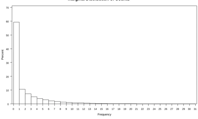
expected to be influential beyond what is normally expected (e.g., statistical power). Each of the four data generation conditions were replicated 500 times resulting in a total of 2000 generated datasets. Figure 3 shows the marginal distribution of the simulated outcome for all 500 replications from Condition 1. Because counts had to be between 0-30, I recoded any counts greater than 30 to missing. This affected a very small percentage of the generated data ( > 99.5% of the generated data generated across all of the conditions had counts between 0-30).
Step 2: Alcohol Measures
Although there are already many different alcohol frequency scales, I also explored whether it was possible to draw on statistics (e.g., GLM theory) to improve ordinal frequency measures for use in standard linear models. This experimental fourth measure was a seven category measure that I created based on a logarithmic transformation. More specifically, I created the 7 categories by dividing the maximum log(day+1) by 7 and creating cutoffs based on increments of that magnitude (See Table 2). For instance, 3.43 divided by 7 is .49, so I created bins using a .49 cutoff for the log(days+1).
Step 3: Scoring Approaches
Three scoring approaches were applied to the ordinal data produced in Step 2. The first two scoring approaches used were the category numbers and median values within each category. The third scoring approach was an experimental approach I propose that draws on the logarithmic transformation. This approach simply takes the log of the median value within each category plus one (e.g., log(median+1)). I derived this experimental scoring method as an attempt to optimize the performance of ordinal scores in standard linear models using statistical theory.
Step 4: Model Fitting
To be consistent with applied research, standard linear regression models were fitted to the ordinal data scored in Step 3. Linear regression models were fitted to data using SAS PROC REG. Using Equation 4, the mean model can be expressed as
2 1 0 2 1 1 i ii x x
μ
generating ZINB model to the count data using SAS PROC COUNTREG to validate data generation.
Simulation Evaluation
I used a series of meta-models to test for the potential interaction of measure-by-scoring approaches and the measure and score main effects. The meta-models were eight separate GEE models with logit link functions, binomial response distributions, and
exchangeable correlation structures (4 effect size conditions by 2 predictors) fitted to binary outcome of Type II error (e.g., 0=No Type II error, 1=Type II error). I used GEE models to account for the correlations among scale-by-scoring combinations fitted the same underlying count data (the same general pattern of results were obtained using random effects
models).The eight models had a total of 6,000 observations because for each of the 500 replications there were 12 lines of data representing the various measure-by-scoring
approaches. I created reference codes for measures and scoring approaches to formally test for the main effects and their interaction. These meta-models were used only to test for omnibus scale-by-scoring effects or scoring and measure main effects when the interaction was non-significant. This was accomplished with Wald test statistics. I did not use any model implied probabilities or odds ratios to evaluate the simulation.
the different ordinal alcohol measures and scoring approaches. Given these conditions, I evaluated my simulation using three criterion.
First, I examined differences in the proportions of significant effects obtained when using the ordinal data and standard regression models compared to the counts fitted to population generating ZINB model. For additional comparison information, I also calculated the standardized regression coefficients for the multiple linear regression models fitted to the ordinal data. I did not do this for the population generating ZINB model because there were not satisfactory computational methods. Second, I examined Type I and II error rates and odds ratios for the various measure-by-scoring approaches compared to the population generating ZINB models. Third, I calculated the proportion of the generated datasets that produced different patterns of effects due to measures and scoring approaches despite having the same underlying count data. For example, assuming the same underlying data and alcohol frequency measure, if x1 was significant using the category number scoring approach but not using median scoring approach, I labeled this as a “different pattern of effects”.
Simulation Summary
Empirical Demonstration
About the NLSY
I employed an empirical demonstration to determine if standard linear models fitted to ordinal alcohol frequency data can lead to different substantive results in practice. I used repeated random samples instead of working with a single dataset as is typically done in empirical demonstrations because I wanted to work with a sample size that is reflective of those commonly observed in adolescent alcohol use studies. The study that I used for this demonstration had a very large sample size of almost 9,000 adolescents and young adults. Using repeated random sampling allowed me to specify a much smaller sample size (n=250) so that my findings would generalize to a broader audience and there was not excessive statistical power. Even without knowing the population generating model, repeated random sampling allowed me to describe my empirical demonstration in terms of proportion of significant effects and the proportion of datasets that had inconsistent patterns of effects caused by measures and scoring approaches.
Data for the empirical demonstration came from the first round of data collection for the NLSY (NLSY97). The NLSY was selected because, unlike most studies, they collected count data for alcohol frequency, which is necessary for my evaluation strategy. Briefly, the NLSY collected extensive information on several domains including educational
experiences, employment data, delinquent behavior, alcohol and drug use, sexual activity, youth's relationships with parents, contact with absent parents, marital and fertility histories, dating, onset of puberty, training, participation in government assistance programs,
expectations, and time use.
8,984 participants ranging in age from 12 to 18 years old. The sample was 51% male and the Race/Ethnicity breakdown was 51.9% Non-black/non-Hispanic, 26% Black, 21.2% Hispanic or Latino, and 0.9% Mixed Race/Ethnicity.
Study Subsample
For the purposes of my project, a subsample was created. The subsample consisted of 4,442 14-16 year old adolescents (51.9% male; 33.2% 14 year olds, 34.1%15 year olds, 32.7% 16 year olds; 35.1% minority). There were very few 12 and 13 year olds (1.3% of the initial sample) and the NLSY did not collect relevant items concerning maternal monitoring for participants that were older than 16 years old so these ages were dropped. Additionally, because this demonstration used standard linear regression models for the analyses,
participants that had missing data on any variables used for the analyses were dropped so that there was a common sample size across all models (11% of the 14-16 year old adolescents were dropped because they were missing on at least one covariate).
Measures
Alcohol Frequency
Alcohol frequency was a single open ended item, “During the last 30 days, on how many days did you have one or more drinks of an alcoholic beverage?”. The responses were
discrete counts ranging from 0-30. Maternal Monitoring
Maternal monitoring was a composite consisting of the mean of three items: “How much does she (mother) know about your close friends, that is, who they are?”, “How much does she (mother) know about your close friends' parents, that is, who they are?”, and “How
items had a five point likert response scale: 0=”Know Nothing”, 1=”Knows Just A Little”, 2=”Knows Some Things”, 3=”Knows Most Things”, 4=”Knows Everything”. The items had a Cronbach’s alpha of .72.
Analytic Strategy
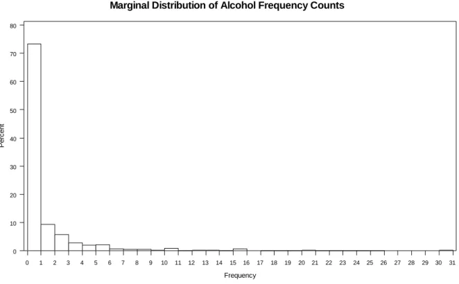
The analytic strategy for this empirical demonstration was the same as the simulation with the exception of Step 1. For the empirical demonstration Step 1 involved taking 1000 random samples of n=250 with replacement from the total subsample of n=4,442. The 1,000 unique datasets subsequently went through Steps 2-4 from the simulation strategy. Figure 4 shows the marginal distribution of alcohol frequency counts for the whole subsample of n=4,442. The linear regression model based on Equation 4 fitted to the data was
4 3 2 1 0 1 i i i ii Age Minority Gender Monitor
μ
For comparison purposes, I fitted a negative binomial (NB) model with the same predictors to the count data, see Equation 5. The NB model provided what should be a more appropriate standard for evaluating the linear regression models fitted to the ordinal alcohol frequency data. I fitted NB models instead of the ZINB models because many of the 1,000 randomly sampled datasets appeared to be consistent with the NB distribution. In these cases, the fitted ZINB models often led to seemingly unstable estimates and convergence
difficulties. Given this, I decided to use the more stable NB models for comparison. Evaluating the Empirical Demonstration
inferences from linear statistical models. First, I calculated the different proportions of significant effects caused by measures and scoring approaches. I also provided the
standardized regression coefficients for the predictor effects in the linear regression model. The results produced from the linear regression models fitted to the ordinal data were compared among each other and to the NB model fitted to the counts. Second, I calculated the proportions of the generated datasets that had different patterns of effects caused by measures and scoring approaches despite having the same underlying count data. These proportions only considered patterns of effects from the linear regression models fitted to the ordinal alcohol frequency data (did not consider the patterns of effects produced by the NB models fitted to the counts).
In sum, the goals of this study were to evaluate the impact of ordinal measures and scoring approaches on our ability to draw valid inferences from linear statistical models. The simulation study provided a highly controlled environment with known population
Results
First, I will present results from the simulation study. I used omnibus Wald tests from the GEE meta-models to assess whether or not there was scale-by-scoring approach
interaction effect (and main effects of scale and scoring, if the interaction was non-significant) on the probability of making Type I and II errors. To untangle the interaction effects, I examined various outcomes including the proportions of Type I and II errors, odds ratios for making Type I and II errors compared the population generating ZINB model, standardized regression coefficients from the linear regression models, and percentages of different patterns of effects. Second, I will present results from the empirical demonstration. Again, I used omnibus Wald tests from the GEE meta-models to generally assess whether or not there was scale-by-scoring approach interaction effect (and main effects of scale and scoring, if the interaction was non-significant) on the probability finding significant effects. I examined the proportions of significant effects, odds ratios for finding significant effects compared the NB models, standardized regression coefficients for the linear regression models, and percentages of different patterns of effects.
Simulation Study
Recovery of Population Generating Values
Table 3 shows the recovery of the population generating values by the ZINB models. The ZINB models showed fair recovery of the parameter estimates across all four effect size
conditions. For example, the mean dispersion parameter (α, which is equivalent to ),
but had average estimates of -.44 in condition 1 (binary predictor, x1, had a medium effect), -.75 in condition 2 (binary predictor, x1, had a small effect), -.73 in condition 3 (continuous predictor, x2, had a medium effect), and -1.09 in condition 4 (continuous predictor, x2, had a medium effect) across the 500 replications. Although the mean point estimate for the inflated zero parameter was biased across conditions, the standard errors were large. This reflected imprecision in the estimates and this is consistent with research that has suggested that parts of these models, including point estimates, can be sensitive to smaller sample sizes (Ghosh, Mukhopadhyay, & Lu, 2006).
Hypothesis 1: Scale-by-Scoring Approach Interaction
First, I evaluated my hypothesis that there would be a scale-by-scoring approach interaction effect on the inferences drawn from linear statistical models. The meta-models described earlier in the Methods section consistently showed a significant scale-by-scoring approach interaction on the probability of Type II errors across the four effect size conditions (for x1: condition 1 χ2(6)=56.94 , condition 2 χ2(6)=27.18 ; x2: condition 3 χ2(6)=56.56, condition 4 χ2
(6)=35.73; p<.0001 for all tests). To help understand these interactions, I examined outcomes based on the raw data from simulation results, not the parameter estimates from the GEE meta-models. Table 4 through Table 7 display the proportion of significant effects, proportion of Type I and II errors, odds ratios for Type I and II errors for the scale-by-scoring combinations compared to the population generating ZINB models, and the standardized regression coefficients across the four effect size conditions.
(e.g., Condition 1: 8pt NIAAA 29%; 11pt 29% ; 7pt log 31%) producing a reduced percentage of Type II errors compared to category number scores (e.g., Condition 1: 8pt NIAAA 40%; 11pt 36%; 7pt log 41%), which had reduced percentage compared to log median scores (e.g., Condition 1: 8pt NIAAA 44%; 11pt 43%; 7pt log 44%). However, this pattern in the scoring approaches did not hold for the five point measure. The percentage of Type II errors using the log median scoring approach (Condition 1: 48%) was slightly less than those for the category number (Condition 1: 51%).
Another way I conceptualized this interaction was by examining how the scoring approaches depended on measures. Results indicated that category scores were more influenced by measures than median and log median scores. More specifically, category number scores that were used with the five point scale led to more Type II errors relative to the other measures than median and log scores. For instance, the difference in Type II errors for category number scores applied to the five point scale versus the eleven point scale (Condition 1: 51% vs. 36%) was three times larger than the difference between these scales for median (34% vs. 29%) and log median scores (Condition 1: 48% vs. 43%). This general trend holds across all conditions for non-zero effects. The impact of the scale-by-scoring approach interaction was relative to the designated effect size (e.g., the discrepancies in Type II error rates for the “small” effect were reduced by roughly one-half). The proportion of significant effects and standardized regression coefficients from Tables 4 through 7 reiterated these findings except they had an inverse relationship with Type II errors. Higher Type II error rates corresponded with a lower proportion of significant effect and smaller
The meta-models did not find effects of scoring approaches, measures, or their interaction on the Type I error rate across the conditions (for all models p > .05). Tables 4 through 7 show that there were no clear differences in the proportion of Type I errors across the various measure-by-scoring approach combinations. Type I error rates were consistently around .03-.05 across conditions. I also tested whether the scale-by-scoring combination could potential induce a spurious interaction between x1 and x2. Results did not support the existence of this interaction in any conditions.
Hypothesis 2 and 3: General Effects of Scoring and Measures
Measures and Scores Leading to Different Patterns of Effects
I evaluated how scores interacted with measures to impact the validity of inferences by identifying whether different scores led to different patterns of effects using the same measure. For example, consider a case in which the eight point NIAAA measure with median scores was used and there was significant effect of x1 and no significant effect of x2. Then, given the same underlying data and eight point NIAAA measure, category scores were applied and there were no significant effects of x1 or x2. This was identified as a “different pattern of effects”. Table 8 shows that in condition 1 and 3, across the four measures between 19-24% had different patterns of effects caused by scoring approaches. In condition 2 and 4, across the measures 15-20% had different patterns of effect caused by scoring. These results indicated that different patterns of effects were often caused by scoring approaches. In all conditions, the five point scale had a slightly higher proportion of inconsistent patterns of effects compared to the other scales.
Similarly, I evaluated the effect of measures on the validity of inferences by identifying whether different measures led to different patterns of effects using the same scoring technique. For instance, consider a case in which the median scores were applied to the eight point NIAAA measures and there was significant effect of x1 and a no significant effect of x2. Then, given the same underlying data and median scores were applied to the five point measure, but there were no significant effects of x1 or x2. This was considered a
“different pattern of effects”. I found that across all conditions, different patterns of effects
measures. Different patterns of effects due to measures occurred less frequently using the log transformation scoring approach (8%-9%).
In sum, this simulation study showed that there was an interaction between scores and measures that led to increased Type II errors. The five point scale depended on scoring in a fundamentally different way than the other scales. More specifically, the five point scale performed worst with category scores whereas this was not the case for the other scales. There was a general trend of median scores outperforming category scores and category scores outperforming log median scores. Additionally, the five point measure was consistently outperformed by the other measures across the scoring approaches. My simulation showed that measures and scores often created different patterns of effects. In sum, these results suggested that scales and scoring approaches likely impact adolescent substance researchers’ ability to test theoretical models through the reduction of statistical
power and changes in patterns of effects.
Empirical Demonstration
I used empirical data from the NLSY to further evaluate my hypothesis that there should be a scale-by-scoring approach interaction effect of the inferences drawn from linear statistical models. The omnibus Wald tests from GEE meta-models described earlier found significant scale-by-scoring approach interactions on the log odds of obtaining a significant effects for each of the four predictors (age: χ2(6)=46.00 , minority: χ2
(6)=77.38 , p<.0001; maternal monitoring: χ2
(6)=20.46, p<.001). The interaction effect for gender was significant, but its magnitude appeared smaller given the high statistical power (χ2
Table 10 displays the proportion of significant effects, odds ratios for obtaining a significant effect for the scale-by-scoring combinations compared to the NB model fitted to the counts, and standardized regression coefficients. These outcomes were based on the empirical results, not the estimated GEE meta-models. For the age and minority effects, the scale-by-scoring approach interaction was driven by a dependency between the five point scale and median scores. For instance, across the eight point NIAAA, eleven point, and seven point log scales there was a general trend of median scores resulting in a smaller proportion of significant effects of age than category and log median scores (i.e., for the 11 point scale: log median 47% and category number 48% vs. median scores 39%). However, the five point scales had systematically lower proportion significant and the difference between the
proportions for category and log median scores versus median scores was smaller (log median and category number 40% vs. median scores 37%).
For the minority effect, this interaction manifested itself in a slightly different way. Across the eight point NIAAA, five point scale, and seven point log measures, the log
and scores impact Type I and II errors because the population generating model was unknown.
I was not able to make conclusive statements about the effects of scoring and scales on the gender predictor because of the small effect size (proportion significant 5-8% across measures-by-score combinations). The maternal monitoring predictor appeared to be more consistent with a main effect of scoring on the proportion significant effects. More
specifically, across all measures, median scores had a smaller proportion of significant effects compared to log median and category number scales (39-40% vs. 48-52%). Setting aside the specific complexities addressed with the interactive effect of scoring approaches and measures, there was a general trend of median scores having a lower proportion of significant effects compared to other scoring approaches. Log median scores and category scores performed quite similarly across the predictors.
I examined how frequently different scoring approaches led to a different pattern of effects using the same alcohol frequency measure. This process was similar to that outlined in the simulation study. For instance, if the eight point NIAAA measure with median scores was used and there was significant effect of age and maternal monitoring but with category scores there was only a significant age effect, this was considered a “different pattern of effects”. Different scoring approaches applied to the same measures and data frequently caused different patterns of effects; 48% of the models using the eight point NIAAA
measure, 41% of using the five point measure, 51% using the eleven point measure, and 45% of seven point log median measure. I also computed how frequently different measures led to a different pattern of effects using the same scoring approach. Results indicated that
scores, 48% of median scores, and 35% of log median. Taken together, these results showed that the patterns of significance for the covariates varied substantially depending on what measures and scoring approaches were used.
Summary of Results
In sum, both the simulation study and empirical evaluation showed that scales and measures interacted to impact inferences drawn from linear models. Results suggested that the five point scale were more sensitive to scoring than the other three scales. Also, in both the simulation study and empirical demonstration, the five point scale almost always had the lowest proportion of significant effects compared to the other scales. However, the patterns of Type II errors, proportions of significant effects, and standardized regression coefficients suggested that the general impact of scores were markedly different in the simulation study compared to the empirical demonstration. Most notably, median scores performed best in the in simulation study whereas they appeared to perform the worst in the empirical
Discussion
I used a comprehensive simulation study and an empirical demonstration to test my set of theoretically generated research hypotheses concerning the effect of ordinal alcohol measures and ordinal scoring approaches on our ability to draw valid inferences from linear statistical models. The results of my project provided support for my three research
hypotheses.
Results from the simulation study and empirical demonstration suggested that measures and scoring approaches interacted to influence inferences drawn from linear statistical models. In the simulation, category number scores performed worse using the five point scale with response categories defined to be dissimilar to a log transformation
compared to if category numbers were applied to the other three scales. The five point scale also had a general tendency to produce lower proportions of significant effects and larger Type II error rates compared to the other scales. Results suggested that it is not only the number of response categories, but also how counts are binned into categories, that impacted the performance of alcohol frequency measures. Although median scores had the lowest proportion of Type II errors in all conditions of the simulation study, the empirical
demonstration showed that median scores led to the smaller proportion of significant effects compared to the other scoring approaches. In both the simulation and empirical
Hypothesis 1: Scale-by-Scoring Approach Interaction
I hypothesized that ordinal alcohol measures and scoring approaches would have an interactive effect on the validity of results obtained from linear models. I predicted that the five point scale should be more influenced by scoring approaches than the other measures because there were fewer response categories and the categories were not closely reflective of the log transformation. Results from my project supported this hypothesis. In the
simulation, I found that with the five point scale category number scores performed the worst whereas log median scores were the worst with the other scales (e.g., highest Type II error rates). Category number scores applied to the five point measure was by far the worst scale-by-scoring approach combination used in the simulation study. For example, in condition 1, 51% of the models fitted with category scores applied to the five point scale led to Type II errors compared to 29% using median scores applied to the 11 point measure. Results from the empirical demonstration indicated that this scale-by-scoring approach interaction may manifest itself in a slightly different way. For instance, the age effect showed that the discrepancy in the proportion of significant effects between category numbers and log median scores versus median scores was less for five point scale than for any of the other three scales.
Statistical theory explains this scale-by-scoring approach interaction effect. Scoring approaches are inherently dependent on the ordinal measures (e.g., category numbers are based on the ordinal bins of measures) and if an ordinal measure does not effectively transform the underlying alcohol frequency counts, the relationships among a set of
relationships among the covariates and the alcohol frequency outcome were likely not linearized as well as with the other three ordinal alcohol scales. Moreover, because category numbers scores are highly dependent on the category bin sizes, I expected that their
performance would be more affected by the poorly defined response categories. This dependency between scoring and how alcohol frequency counts are binned into ordinal categories has not been identified previously in the adolescent alcohol use literature. To my knowledge, this is the first study to explicitly examine how ordinal scales and scoring approaches interact in linear statistical models.
Hypothesis 2: Effect of Scoring
Beyond the scale-by-scoring interaction effect, I hypothesized that category and log median scores should generally outperform median scores (except with the five point
measure) because they are better suited for linearizing the relationships among the covariates and ordinal alcohol frequency outcome. I found that ordinal scoring approaches applied to binned counts have a large effect on our ability to draw valid inferences from linear statistical models. I was unable to define a clear optimal scoring approach that was robust across the simulation study and empirical demonstration. In the simulation study, the median scoring approach outperformed the category number and log median scoring approaches (e.g., higher proportion of significant effects, lower Type II error rates, and highest standardized
regression coefficients) across the four conditions.
there was a highly significant association whereas the ordinal category scores led to a non-significant association. Findings like this have caused biostatisticians to recommend
assigning scores that are reflective of true distance between categories such as median values (Agresti, 2002). However, supporting my original hypothesis, the results from the empirical demonstration are in direct evidence of the median approach being outperformed by the category number and log median approaches (e.g., lower proportion of significant effects and smaller standardized regression coefficients). This trend cannot be verified because I did not know the population generating model for the empirical data. However, these findings have led me to believe that other characteristics of adolescent alcohol data not considered in this project such as different underlying distributions (e.g., zero-inflated negative binomial, negative binomial, and censored negative binomial) may interact with scoring approaches to affect the results produced in these models.
Another important finding in both the simulation study and empirical demonstration was that, given the same underlying count data and alcohol frequency measure, different scoring approaches frequently produced differing patterns of effects. This finding reaffirms related research on different patterns of statistical significance due to ordinal scoring from other fields such as Graubard and Korn (1987). Taken together, these findings showed that ordinal scoring methods play an integral role in testing theoretical models of adolescent substance use using linear models.
Hypothesis 3: Effect of Measures
In my simulation study, all four of the alcohol frequency scales showed high Type II error rates across all conditions, indicating that standard alcohol measures failed to find effects that truly exist. However, the ordinal scales did not frequently lead to Type I errors. Although the differences among the scales were not always large, the five category scale consistently performed the poorest (e.g., lowest proportion of significant effects, highest Type II error rate, smallest standardized regression coefficients) while the other three alcohol frequency scales performed comparable across the four effect size conditions.
The poorer performance of the five category scale in relation to the other scales was expected for two reasons based on prior research (e.g., MacCallum, et. al, 2002; Taylor, West, & Aiken, 2006). First, the five point scale had the fewest response categories, which is associated with an assortment of negative statistical consequences such as reduced statistical power and effect sizes. Second, the five categories deviated from a viable transformation (e.g., log transformation) more than the other three measures. The impact of how counts were binned is consistent with what Generalized Linear Model theory suggested (e.g., count outcome are often modeled with a log link function; McCullagh, & Nelder, 1989). The seven point log, eight point NIAAA, and 11 point measures likely performed the same because they each had a moderate to large number of reasonably defined response categories (e.g., bin size increased as the response category got higher).
1991). My study was the first to generalize these findings to a process of binning underlying counts into ordinal categories in the context of adolescent alcohol use.
Implications and Recommendations for Applied Research
My findings have several implications for applied research. The results showed that measures and ordinal scoring approaches can sometimes interact in unpredictable ways to influence the researchers’ ability to validly test substantive hypotheses. My study was the first to explicitly show that the performance of alcohol frequency measures depends not only on the number of categories, but also how the open ended alcohol frequency counts are binned. My study was also the first to empirically examine the strong influence of scoring on substantive findings. I clearly demonstrated that both measure and scoring approach can substantially lower statistical power. Equally concerning is the idea that a researcher can have one data set and apply multiple scoring approaches, yet come to completely different substantive interpretations. There was no conclusive evidence that measures and scores lead to increased Type I errors, but that does not mean it cannot happen in practice. For example, in the empirical demonstration, the minority effect actually had a higher proportion of
significant effects using linear models fitted to ordinal data than the negative binomial model fitted to the counts. This trend suggested that elevated Type I errors may arise in practice.
frequency data on a single ordinal scale and knowingly, or unknowingly, change their findings solely because of how the alcohol frequency data are scored. This type of risk is typically nonexistent with ordinal alcohol measures because the categories are usually defined on a survey a priori.
Based on the findings of this study, I offer four recommendations for adolescent alcohol use researchers. First, it is vital that methodological work like I have conducted in this project be disseminated so that researchers can become aware that the quantitative characteristics of alcohol measures and ordinal scoring approaches can cause substantively different model results. Second, researchers should strongly consider collecting open-ended count data and modeling the counts with appropriate nonlinear models (e.g., Poisson,
Finally, to minimize the negative impact of scoring approaches on linear models, I recommend doing a two-step sensitivity evaluation. First, researchers should perform a thorough exploration of their data using graphical and descriptive techniques with different ordinal scoring approaches. Descriptive explorations should involve examining the basic properties of the alcohol frequency data independently (e.g., mean, standard deviations, tests of distributions) and conditional on covariates (e.g., correlations, conditional means).
Graphical explorations such as scatter plots fitted with smoothed curves and other
visualization of functional form are essential to ensuring that ordinal scoring approaches are not inducing nonlinear relationships between the covariates and the outcome (median scores and scores based on poorly defined measures should be of greatest risk for this). Researchers should fit multiple models to different ordinal scores to assess sensitivity. If results are the same across these models, researchers can feel confident in their pattern of results under the assumption that all of the models are not consistent and wrong. If the results differ,
researchers should refer back to the data exploration from step 1 and consider what pattern of effects is most consistent with substantive theory so that they can make the best decision possible. Researchers should always inform the reader of their scoring method, define the response categories of their measures, and note if their findings are sensitive to different scoring approaches.
Limitations and Future Directions
showed the impact of measures and scores results using existing data, but there was no way to know which scoring method and measure was best because the population generating model was unknown. Findings from my project cannot be generalized directly to the
longitudinal setting because scores and measures likely interact in more complicated ways to impact our ability to accurately test theoretical models of adolescent alcohol use over time. I did not include a condition where I fit the ordinal alcohol frequency data with ordinal
statistical models in my project. This is not standard practice in applied research and I currently cannot comment on the performance of these types of statistical models for adolescent substance use data.
Possibly the most important direction is determining whether or not researchers should collect adolescent substance use data on an ordinal scale. Ordinal measures may help to eliminate some unreliability in participants’ recall of the actual count of the number of
days they have used alcohol, but it is unclear if this assumed improvement in reliability offsets the statistical consequences of fitting linear models to ordinal data (e.g., increased Type II errors). Future studies should clarify whether or not collecting more unreliable count data that can be modeled in appropriate nonlinear statistical models has added benefits over the current standard practices in measuring and model adolescent substance use data.
Currently, the field of adolescent substance use has failed to fully capitalize on several recent advances in nonlinear statistical models for count data such as Poisson, Negative Binomial, and various techniques for Zero-inflated data. These novel nonlinear methods have the potential to improve our ability to draw accurate inferences from statistical models, while at the same time increase the breadth of hypotheses that can be formally tested compared to current practices. However, in order to capitalize on the flexibility of these innovative models, we must first justify that the collection of count data over more commonly collected ordinal data.
Conclusion
the results obtained from linear statistical methods (e.g., Graubard and Korn , 1987), my study explicitly compared multiple methods and showed that scores depend on measures and likely other unknown factors (e.g., underlying distributions). Existing advice on ordinal scores from the field of biostatistics recommends using median scores (Agresti, 2002), but my study suggested that median scores may not always be the best choice for all research settings. Third, my study outlined how measures and scoring approaches can interact in complicated ways. For instance, category scores applied to the five point scale with poorly defined ordinal categories led to far more Type II errors than category scores applied to any of the other three measures. Moreover, pairing different score-by-measure combinations on the same underlying data will often lead to researcher drawing substantively different inferences from linear models. Taken together, these findings clearly showed that measures and ordinal scoring approaches have the ability to affect adolescent alcohol researchers’
Table 1.
Four alcohol frequency scales for a past 30 day time frame
How many days in the past 30 days have you had one or more drinks?
8 Point NIAAA Scale
5 Point Scale
11 Point Scale
7 Point Log Scale
7. 28-30 days 6. 18-27 days 5. 10-17 days 4. 6-9 days 3. 4-5 days 2. 2-3 days 1. 1 days 0. 0 days
4. 24-30 days 3. 16-23 days 2. 6-15 days 1. 1-5 days 0. 0 days
10. 25-30 days 9. 20-24 days 8. 15-19 days 7. 11-14 days 6. 8-10 days 5. 6-7 days 4. 4-5 days 3. 3 days 2. 2 days 1. 1 day 0. 0 days
48
Table 2.
Experimental seven point measure based on the log transformation.
C1 C2 C3 C4 C5 C6
Days 0 1 2 3 4 5 6 7 8 9 10 11 12 13 14 15
Log(day+1) 0 .70 1.10 1.39 1.61 1.79 1.95 2.08 2.20 2.30 2.40 2.48 2.56 2.63 2.71 2.77
C6 (cont.) C7
Days 16 17 18 19 20 21 22 23 24 25 26 27 28 29 30