RESEARCH ARTICLE
10.1002/2014JC010104
Exploiting satellite earth observation to quantify current global
oceanic DMS flux and its future climate sensitivity
P. E. Land1, J. D. Shutler1, T. G. Bell1, and M. Yang1
1Plymouth Marine Laboratory, Prospect Place, West Hoe, Plymouth
Abstract
We used coincident Envisat RA2 and AATSR temperature and wind speed data from 2008/2009 to calculate the global net sea-air flux of dimethyl sulfide (DMS), which we estimate to be 19.6 Tg S a21. Our monthly flux calculations are compared to open ocean eddy correlation measurements of DMS flux from 10 recent cruises, with a root mean square difference of 3.1lmol m22day21. In a sensitivity analysis, we varied temperature, salinity, surface wind speed, and aqueous DMS concentration, using fixed global changes as well as CMIP5 model output. The range of DMS flux in future climate scenarios is discussed. The CMIP5 model predicts a reduction in surface wind speed and we estimate that this will decrease the global annual sea-air flux of DMS by 22% over 25 years. Concurrent changes in temperature, salinity, and DMS concentra-tion increase the global flux by much smaller amounts. The net effect of all CMIP5 modelled 25 year predic-tions was a 19% reduction in global DMS flux. 25 year DMS concentration changes had significant regional effects, some positive (Southern Ocean, North Atlantic, Northwest Pacific) and some negative (isolated regions along the Equator and in the Indian Ocean). Using satellite-detected coverage of coccolithophore blooms, our estimate of their contribution to North Atlantic DMS emissions suggests that the coccolitho-phores contribute only a small percentage of the North Atlantic annual flux estimate, but may be more important in the summertime and in the northeast Atlantic.1. Introduction
The global oceans are the largest natural source of atmospheric sulfur through the emission of the gas dimethyl sulfide (DMS) [Bates et al., 1992]. Derived from the growth and decay of phytoplankton, DMS is ubiquitous in the surface ocean, with dissolved concentration grossly supersaturated relative to the overly-ing air, resultoverly-ing in consistent emission to the atmosphere. Once in the marine atmosphere, the oxidation of DMS leads to sulfur dioxide, sulfuric acid, and sulfate aerosols, among other products. These acidic and hygroscopic species affect atmospheric chemistry [Charlson and Rodhe, 1982], and contribute to the nuclea-tion of new particles as well as the growth of existing particles to cloud condensanuclea-tion nuclei (CCN). Such condensation nuclei affect the Earth’s radiation budget (and thus climate) by directly scattering sunlight and indirectly influencing cloud physics and albedo [Charlson et al., 1987].
Despite increasing anthropogenic sulfur emissions, DMS remains the predominant source of sulfur mass to the remote marine atmosphere [Yang et al., 2011b]. There is, however, much debate over the exact role that DMS plays in regulating our climate.Gunson et al. [2006] modeled a 0.8C cooling for a doubling of DMS
emission, and a 1.6C warming for a halving of DMS emission. Furthermore, their modeled DMS emission
increases over time in response to warming and decreases in response to cooling, consistent with a nega-tive climatic feedback. Other studies suggest less climate sensitivity to DMS. For example,Boucher and Loh-mann[1995] andWoodhouse et al. [2010] found the radiative properties of clouds to depend more on total sulfate and cloud droplet number concentrations (partly anthropogenic) than on DMS and naturally derived sulfate. Similarly,Quinn and Bates[2011] argued that the climate regulation by DMS is weak mostly because of other sources of CCN, e.g., sea salt and organics, whileClarke et al. [2013] found the main source of CCN in the marine boundary layer (MBL) to be entrainment of preexisting aerosols from the free troposphere rather than nucleation and growth within the MBL. The impact of DMS on clouds is thought to be most sig-nificant in regions with minimal competitions from anthropogenic CCN [Twomey, 1991].Boucher et al. [2003] showed large spatial heterogeneity in their modeled indirect radiative forcing due to DMS-derived aerosols, varying from close to zero to25 Wm22
.Woodhouse et al. [2013] recently demonstrated highly variable sensitivity of CCN production as a function of DMS emission and argued for the importance of Key Points:
Global sea-air fluxes of DMS are quantified
Effect of 25 years of modelled climate change is dominated by reduced wind
Coccolithophores are estimated to have a small effect on DMS fluxes
Supporting Information: Readme Figure S1 Figure S2 Figure S3 Figure S4 text01 Correspondence to:
P. E. Land, [email protected]
Citation:
Land, P. E., J. D. Shutler, T. G. Bell, and M. Yang (2014), Exploiting satellite earth observation to quantify current global oceanic DMS flux and its future climate sensitivity,J. Geophys. Res. Oceans,119, 7725–7740, doi:10.1002/ 2014JC010104.
Received 15 MAY 2014 Accepted 15 OCT 2014
Accepted article online 20 OCT 2014 Published online 19 NOV 2014
monitoring of future changes in spatial DMS distributions.Six et al. [2013] argued that ocean acidification would reduce DMS emissions, resulting in a radiative forcing of 0.4 Wm22.
Previous estimates for the present day global sea-to-air flux of DMS range from 15 to 33 Tg S a21[Elliott, 2009;Kettle and Andreae, 2000;Simo and Dachs, 2002]. Based on the most recent DMS climatology,Lana et al. [2011] estimated a mean annual emission of 28.1 Tg S a21, with a range from 17.6 to 34.4 Tg S a21 depending on the choice of transfer velocity parameterization (see subsection 4.1). Predictions of future DMS emission vary significantly, especially on a regional scale [Cameron-Smith et al., 2011;Halloran et al., 2010] due to combined uncertainties in the changes of seawater DMS concentration, winds, temperature, etc. Observations and recent modeling studies indicate that the concentration of DMS in surface seawater is the net result of rapid but variable biological production and consumption processes [Galı et al., 2013]. A small perturbation in DMS source or sink can significantly influence the amount of seawater DMS available for air-sea exchange.
Earth observation (EO) data from satellites have the potential to help predict regional changes in DMS emis-sions. In the Arctic, where in situ observations are rare, the use of EO data underpinned by field data is cur-rently the most feasible way of reliably monitoring sea-air gas fluxes. EO data have previously been used to derive sea-air fluxes of CO2at the global scale [e.g.,Boutin et al., 2002], and the improved quasi-global
avail-ability of EO data has facilitated recent studies of CO2sea-air exchange over a substantial area of the Arctic
Ocean [Arrigo et al., 2010;Else et al., 2008]. In comparison, the use of EO data to study sea-air gas exchange of trace gases including DMS is novel. Such methods have the potential to improve our understanding of the global sulfur cycle and its impact on climate.
One specific example of EO data utility is the potential to constrain the contribution to the global DMS flux from coccolithophore blooms. Algal species produce a large range of intracellular dimethylsulfoniopropio-nate (DMSP), which is the major algal precursor to DMS [Keller et al., 1989]. Diatoms are low DMSP/DMS pro-ducers, with intracellular DMSP on the order of 0.86 mmol/mol C [Stefels et al., 2007]. In sharp contrast, the haptophyte phytoplankton group, which contains coccolithophores, has a higher intracellular DMSP con-tent (11 mmol/mol C), which is second only to dinoflagellates (22 mmol/mol C) [Stefels et al., 2007]. In the open ocean, certain coccolithophore blooms are clearly detectable by satellites. Some blooms have been observed to produce substantially elevated DMSP and DMS concentrations and are thought to contribute substantially to the DMS sea-to-air flux [Malin et al., 1993;Matrai and Keller, 1993;Steinke et al., 2002a]. Globally and regionally, predicting future DMS emissions requires predictions of (1) surface seawater DMS concentration; (2) changes in forcing parameters (e.g., wind speed, SST, salinity), and (3) the sensitivity of DMS flux to these forcing parameters.
Here we use spatially and temporally coincident EO data from the European Space Agency’s (ESA) Envisat satellite to estimate the global flux of DMS in 2008 and 2009. We then evaluate the sensitivity of sea-air DMS exchange in the global ocean to changes in temperature, salinity, wind speed, and aqueous DMS con-centration, both using fixed scalar changes in conditions and arising from future climate model scenarios.
2. Methods
2.1. Data Inputs
We used EO data from Radar Altimeter 2 (RA2) and Advanced Along Track Scanning Radiometer (AATSR) on ESA’s Envisat satellite. RA2 is an altimeter that can provide estimates of wind speed at 10 m height (U10)
with a small surface footprint. In the absence of clouds, AATSR provides estimates of sea surface skin tem-peratureSSTskinover a much wider swath [Donlon et al., 2007]. The fields of view of the two instruments
overlap, providing spatially and temporally coincident measurements. Globally, RA2 has an error standard deviation of 1.25 ms21and a bias of20.28 ms21[Queffeulou et al., 2010], while AATSR has a standard devia-tion of 0.16C and bias of10.2C [O’Carroll et al., 2008]. We processed the RA2 and AATSR data for 2008–
2009 using standard ESA methods and binned them to a 131geographic grid, see [Land et al., 2013] for
details.
Climatological values of the bulk concentration of DMS in surface seawater (DMSw) were obtained on a
131grid from theLana et al. [2011] climatology, while climatological salinity values were obtained on the same grid from the NOAA National Oceanographic Data Center (http://www.nodc.noaa.gov/OC5/
WOA09/pr_woa09.html). Global daily air pressure fields were provided by the European Centre for Medium-range Weather Forecasting (ECMWF) operational data set (N80 Gaussian gridded analysis on surface levels; ERA-40 format, 6 h fields). The pressure data were reprojected from their original 2.532.5grid to the 1
31grid using linear interpolation. Daily sea ice coverage data were provided by the Operational Sea
Sur-face Temperature and Sea Ice Analysis (OSTIA) system [Donlon et al., 2011;Stark et al., 2008] based on the EUMETSAT Ocean and Sea Ice Satellite Application Facility (OSI-SAF) daily analyses. These daily global OSTIA sea ice coverage data were averaged from their original 0.0530.05grid to the same 131grid. We
used a 409632048 global land mask (0.0930.09) to determine the proportion of land by area in each
131pixel. The land mask is needed to calculate the net fluxes and the use of a higher spatial resolution
subgrid for the land mask gives a more accurate representation of the integrated flux from coastal pixels.
2.2. Calculating Sea-Air DMS Fluxes
We estimated the sea-to-air flux of DMS (F) inlmol S m22day21as the product of the gas transfer velocity,
Kw(cm h21), and the difference in DMS concentration (nM) between the base [DMSaqw] and the top
[DMSaq0] of the mass boundary layer at the sea surface, multiplied by 0.24 to convertKwinto m day21:
F50:24KWDMSaqw2DMSaq0: (1)
[DMSaqw] is set to the bulk concentrationDMSwfromLana et al. [2011], while [DMSaq0] is set toH DMSa, where
His the dimensionless Henry’s Law solubility from liquid to gas, calculated as a function of temperature and salinity using the methods ofJohnson[2010], andDMSais the bulk concentration of DMS in air, giving
F50:24KwðDMSw2H3DMSaÞ: (2)
DMSa(units 10
29
mol/L of air) is estimated asDMSw(in units of nM) divided by 400, where both
concentra-tions are expressed in equivalent units. The dimensionless water/air ratio of 400 represents an order of mag-nitude value based on observations from 10 open ocean cruises (see Table 1). This fixed ratio clearly does not capture variations on small temporal or spatial scales, but is intended to be broadly representative of the ratio on a regional to global level. The relative importance of theH3DMSaterm varies with
tempera-ture (and slightly with salinity) due to changes inH. In 2 years of monthly global data at 1spatial resolution,
H3DMSavaries from 2% ofDMSwin the warmest waters to 7% in the coldest.
Kwis the reciprocal of the total resistance to gas transfer on both sides of the air/water interface [Liss and
Slater, 1974], given by
1=Kw51=kw1H=ka (3)
Daily maps of the in-water gas transfer velocitykwwere derived from theSSTskinandU10data using the
wind-based parameterization ofGoddijn-Murphy et al. [2012], who compared all available DMS eddy correla-tion measurements of gas-transfer velocity with altimeter-derivedU10:
Table 1.Summary of DMS Concentrations and Fluxes From 10 Cruises, Compared to Fluxes From This Study
Cruise TAO PHASE BIO Knorr 06 DOGEE aa DOGEE ba Knorr 07 SO GasEx VOCALS Knorr 11
Location Equatorial Pacific
North Pacific Sargasso Sea South Pacific Northeast Atlantic Northeast Atlantic
North Atlantic Southern Ocean Southeast Pacific
North Atlantic
Latitudeb 2
1 5 30 216 43 54 48 251 220 50
Longitudeb 2
98 2179 266 2106 217 211 251 238 280 245
Time Nov 2003 May–Jun 2004 Jul–Aug 2004 Jan 2006 Jun–Jul 2007 July 2007 July 2007 Mar–Apr 2008 Oct–Nov 2008 Jun–Jul 2011
DMSwc 2.6 (0.8) 1.7 (0.7) 2.6 (0.4) 3.8 (2.2) 1.2 (0.6) 6.9 (3.1) 2.5 (1.1) 1.6 (0.7) 2.8 (1.1) 4.1 (2.0)
DMSac 0.0064 (0.0020) 0.0036 (0.0020) 0.0056 (0.0022) 0.0140 (0.0152) 0.0053 (0.0034) 0.0203 (0.0073) 0.0125 (0.0087) 0.0052 (0.0024) 0.0024 (0.0021) 0.0167 (0.0127)
DMSw/DMSa 406 470 464 271 226 340 200 308 1120 245
In Situ Fluxd
7.1 (3.7) 5.1 (3.1) 6.2 (2.4) 12.1 (15.0) 2.7 (2.4) 18.1 (9.4) 5.9 (4.9) 2.9 (2.1) 3.4 (1.9) 7.6 (7.6)
EO Fluxe
3.2 (21.1) 5.0 (0.0) 5.1 (20.5) 8.8 (20.2) 6.6 (1.6) 12.0 (20.6) 2.5 (20.7) 2.6 (20.1) 4.9 (0.8) 6.4 (20.2) Publication Huebert
et al. [2004]
Marandino et al. [2007]
Blomquist et al. [2006]
Marandino et al. [2009]
Huebert et al. [2010]
Huebert et al. [2010]
Marandino et al. [2008]
Yang et al. [2011a]
Yang et al. [2009]
Bell et al. [2013] a
These two are the same cruise but two distinct water masses. b
Cruise Mean, Degrees N or E. c
Cruise Mean,lmol m235nM. d
Cruise mean (standard deviation),lmol m22 day21
. e
kw5ð2:2U1023:4Þ
Sc
660 20:5
; (4)
whereScis the Schmidt number of DMS, calculated as a function of temperature and salinity using the
methods ofJohnson[2010]. We calculatedkafor DMS as a function of wind speed and temperature using
the methods ofJohnson[2010].
2.2.1. Net DMS Fluxes
Using equations (2–4), we calculated the fluxFper unit area of open water. Land and sea ice coverage data were used withFto calculate the net DMS flux from a 131grid cell. Open water area in a given
cell was calculated by subtracting land surface area and sea ice surface area, if any, from the cell. Follow-ing theTakahashi et al. [2009] approach for CO2, we considered<10% sea ice coverage to have a
negligi-ble effect on the DMS flux from a cell, and the calculated flux was unmodified. Sea ice coverage>90% still allows some flux of DMS due to leads, polynyas etc. (where sea-air DMS fluxes may be very strong,
Else et al. [2011]), so in this case coverage was set to 90%. MultiplyingF(per unit area) by the remaining ice free ocean area gives the net DMS flux from the cell. This differs from the methodology ofLana et al. [2011], who set DMS flux to zero if sea ice coverage exceeded 75%, neglecting ice effects otherwise. In 2 years of monthly global 1gridded data, the RMS difference in the annual hemisphere-integrated flux
between the two methods of dealing with partial ice cover is negligible on a global scale (0.003 Tg S a21
in the northern hemisphere and 0.02 Tg S a21in the southern hemisphere – compare with figures in
Table 3).
2.2.2. Missing Data
In a given cell on a given day, it may be that not all the required data are present. RA2 has a small footprint, so daily coverage of RA2 data is generally smaller than that of AATSR. AATSR is vulnerable to cloud contami-nation, so it is quite rare for both data sets to give coincident valid data. The salinity andDMSwdata sets are
also incomplete, with a small amount of missing data around some coastlines. To address this problem, we adopted a hierarchical strategy:
1. If all daily composite data sets are valid at a given position, we use these values; 2. If RA2 or AATSR daily data are missing, we use the monthly composite of that data set.
3. If monthly composite data are missing, we use a composite of that month over the whole time series (currently 2 years).
4. If time series composite data are missing, in the case ofU10, we substituteU10from the daily ECMWF
data. IfSSTskinis missing, the cell flux is not directly calculable. The same is true ifDMSworSis missing,
but this only happens for a very small number of pixels around coastlines, where land masks differ slightly. In these cases, we estimate the cell flux as the monthly average flux in the corresponding 10 latitude band and apply it to the cell. This averaging occurs for 2.2% of the global open water area and 17% of the area in the Arctic over the 2 years.
2.3. Sensitivity to Temperature, Salinity, Wind Speed, and DMS Concentration
We initially variedSSTskin, salinity, U10andDMSwindependently and uniformly over all months and
positions. Though these are not realistic scenarios, they give us a simple insight into the sensitivity of the global flux to changes in individual climate variables. In order to give a more realistic simulation of the effects of predicted climate change, we then used output from the fully coupled ocean-atmosphere Met. Office Hadley Centre Earth System model HadGEM2-ES [Collins et al., 2008] down-loaded from version 5 of the Coupled Model Intercomparison Project (CMIP5), using the RCP8.5 sce-nario [Taylor et al., 2012]. This makes monthly global predictions from 2006 to 2100 assuming a scenario of high anthropogenic CO2emissions. We considered variations inSST, salinity,U10, and
DMSw. The modelSSTis the temperature a few metres below the sea surface, notSSTskin. However,
the difference is a few tenths of a degree, averaging 0.14C for wind speeds greater than 6 ms21 [Donlon et al., 2002], so the temporal changes described in subsection 3.2 are largely unaffected. Each parameter was reprojected to the 131 grid and averaged over 6 years in each month of the year. The data for 2006–2011 were then compared with those for 2031–2036 to estimate the effect of 25 years of change. Averaging over 6 years reduces the effect of transient features in a given year, such as the El Ni~no-Southern Oscillation. We used pixel by pixel changes in this case rather than a uniform
global change because there is strong spatial variability, especially in salinity,U10andDMSw, which
exhibit significant regions of both positive and negative trends.
The sensitivity of DMS flux to plausible changes in each of the four parameters was investigated by applying 25 years of change to one parameter while keeping the others fixed at their original values.SSTvariations were applied tokw,ka,Hand henceFthrough the temperature dependence ofSc(kais not expected to
have a large temperature dependence because the airside Schmidt number is largely temperature inde-pendent). For consistency, salinity variations were applied tokw,Hand henceFthrough the small salinity
dependences ofScandH, though this was not expected to have much effect. The salinities at the surface
and at a depth of a few meters were assumed to covary.U10andDMSwchanges were applied as
percen-tages, since in both cases variations can be negative or positive and values can be close to zero.U10
varia-tions were applied tokwandka, andDMSwvariations were applied directly in equation (2). Finally, we
applied 25 years of change to all four parameters (SST, salinity,U10, andDMSw) simultaneously.
This analysis enabled us to gain insight into the impact of plausible changes in temperature, salinity, wind speed, and aqueous DMS concentration from 2006–2011 to 2031–2036.
2.4. Contribution of Coccolithophores to the North Atlantic DMS Flux
TheLana et al. [2011] climatology was constructed from all available data and no overarching sampling strategy was employed to coordinate the data collection. Some past research activities have focussed on reduced sulfur cycling and certain fieldwork thus specifically targeted coccolithophore blooms [e.g.,Steinke et al., 2002b]. Other DMS data have been collected along transect lines, objectively analysing whatever sea-water masses are encountered. Bloom features thus have the potential to be underrepresented or overre-presented within the climatology, which is not scaled to account for the spatial and temporal frequency of phytoplankton blooms.
The coccolithophoreEmiliania huxleyiis an ideal phytoplankton species for Earth Observa-tion. When the plankton grow and divide at a high rate, they shed their calcium carbonate plates (liths) into the surrounding seawater [Paasche, 2001]. In bloom conditions, the liths create a strong backscattering signal that can be observed by satellite remote sensing [Balch et al., 1991], and can have a significant local effect on radiative forcing [Gondwe et al., 2001]. Recent work has facilitated the routine identification of coccolithophore blooms in the North Atlantic [Shutler et al., 2010].Shutler et al. [2013] used this approach to estimate the proportion of time and space that coccolitho-phore blooms are present within the North Atlantic (75W–11E, 35–68N), see Table 2.
Observations of surface water DMS values within phytoplankton blooms containing high coccolithophore cell density range between 4.8 and 25.0 nM (Table 1). How long this Table 3.Annual Mean DMS Flux (Tg S a21
) per 10 Degree Latitudinal Band in 2008–2009, Compared With the Climatology ofLana et al. [2011]
Latitude 2008–2009 Mean Flux Climatology
90–80N 0.0 0.0
80–70N 0.1 0.1
70–60N 0.2 0.2
60–50N 0.6 0.9
50—40N 0.9 1.5
40–30N 1.0 1.5
30–20N 1.1 1.4
20–10N 1.8 2.6
10–0N 2.1 2.6
0–10S 2.1 2.2
10–20S 2.5 3.5
20–30S 2.1 3.0
30–40S 1.9 2.7
40–50S 1.6 2.8
50–60S 1.1 2.1
60–70S 0.5 0.9
70–80S 0.1 0.1
80–90S 0.0 0.0
Northern hemisphere 7.8 10.8
Arctic (north of 66N) 0.2
-Global 19.6 28.1
Table 2.Monthly Coverage ofE. HuxleyiBlooms in the North Atlantic (75W–11E, 35–68N) and Northeast Atlantic (40W–11E, 60–
68N) During April–Septembera
Coverage (%)
April May June July August September Annual
North Atlantic 0.003 0.08 0.29 0.95 0.44 0.14 0.16
Northeast Atlantic 0.003 0.005 0.36 3.7 2.8 0.87 0.65
a
increase in DMS is sustained over the course of a coccolitho-phore bloom is not well known. We combined satellite-derived spatial coverage of North Atlantic coccolithophore blooms (calculated using the methods ofShutler et al. [2013] and summarized in Table 2) with a range of estimates of the increase in DMS levels due to the bloom and the duration of the increased DMS, to esti-mate coccolithophore bloom-driven sea-to-air DMS flux over plausible ranges of bloom DMS enhancement and duration, in the hope that future work will constrain these ranges. We calculated the increase in annual DMS flux assuming that blooms increase DMS by 5, 15, and 25 nM while a bloom is iden-tified from satellite in a given pixel, and this effect is assumed to continue for 1–20 days, day 1 being the day of satellite detection.
3. Results and Discussion
3.1. Integrated DMS Flux
The mean daily open water DMS fluxFover 2008–2009 is shown in Figure 1, and its seasonal variations are shown in Figure 2, which also shows eddy correlation measurements of DMS flux from 10 cruises (cruise mean, not seasonal mean). Cruises that overlap two seasons are shown in both. The annual integrated DMS fluxes over 10latitude bands are listed in Table 3, along with the annual global, northern hemisphere, and
Arctic (north of 66N) DMS fluxes. These figures are compared with the equivalent climatological values
fromLana et al. [2011]. The cruise data shown in Figure 2 are summarized in Table 1, which also shows the mean EO modeled DMS fluxF(‘‘EO Flux’’) over the cruise months in 2008–2009 in a 535window around
the mean cruise position.
Eight out of 10 of the EO fluxes are less than the in situ fluxes, implying a possible bias. However, all but two of the differences are less than the standard deviation of in situ flux, and a paired t-test reveals no sig-nificant difference between the two (p50.16). As a further check, we estimated the bias between the two data sets by calculating the mean of each, weighted by the reciprocal of the standard deviation of in situ flux. The in situ mean was 5.2lmol m22day21and the EO mean was 4.9lmol m22day21, both with a standard error of 1.1lmol m22day21, implying an EO underestimate of 7628%.
The root mean square difference between the mean in situ fluxes and the mean EO flux is 3.1lmol m22 day21, similar to the global mean flux of 3.5lmol m22day21calculated from our data. Much of this vari-ability can be accounted for by differences in DMS between ship and climatology (RMS difference in DMS is 32%, equating to a 32% difference in flux, see Section 3.2) and differences in wind speed between ship and satellite (RMS difference in wind speed is 16%, equating to a 21% difference in flux), while SST has much less effect (RMS difference of 0.9C, suggesting a flux difference of 2.5%).
Lana et al. [2011] found a global flux of 28.1 Tg S a21, while our analysis suggests a global flux of 19.6 Tg S a21. In the northern hemisphere,Lana et al. [2011] estimate a flux of 10.8 Tg S a21while we find 7.8 Tg S a21. A significant part of these differences can be ascribed to the choice of flux parameterization. This study uses a linear relationship betweenkwand wind that has been derived from direct measurements of DMS flux [
Goddijn-Murphy et al., 2012], whileLana et al. [2011] use the quadratic relationship ofNightingale et al. [2000], resulting in increased fluxes at high wind speeds. It has been proposed that the difference in the functional form of these gas exchange parameterizations results from bubble-mediated gas transfer at high winds, which is enhanced for insoluble gases [Woolf et al., 2007]. Highly insoluble gases were used to estimate the nonlinear relationship betweenkand wind speed inNightingale et al. [2000]. In contrast, DMS is moderately soluble, and
Figure 1.Annual mean sea-air DMS flux (lmol S m22 day21
recent eddy correlation measurements at high wind speeds do not suggest gas-transfer velocity enhancements at high-wind speeds [Bell et al., 2013;Goddijn-Murphy et al., 2012;Marandino et al., 2009;Yang et al., 2011a]. When we recalculate our fluxes usingNightingale et al. [2000], we obtain a global flux of 23.1 Tg S a21and a northern hemisphere flux of 8.8 Tg S a21.
3.2. Sensitivity to Predicted Changes in Temperature, Salinity and Wind Speed
In the initial sensitivity study, we changed a single parameter by a fixed amount, independent of location or month. In all cases, we found the effect to be linear (r2>0.997), so only the effect per unit change in the parameter is quoted. The effect of increasingSSTskinuniformly was an increase in mean global DMS flux of
0.55 Tg SC21(12.8%C21). The effect of increasing salinity uniformly was a decrease in global flux of 0.028 Tg S PSU21(20.14% PSU21). The effect of increasing log(U10) uniformly (i.e., increasingU10by a
uni-form proportion) was an increase in global flux of 25 Tg S per unit of (natural) log(U10), hence a 1% increase
in U10results in an increase in global flux of 0.25 Tg S (11.3%), reflecting the approximately linear
relation-ship between flux and wind speed. The effect of increasing log(DMSw) uniformly was an increase in global
flux of 20 Tg S per unit of (natural) log(DMSw), hence a 1% increase inDMSwresults in an increase in global
flux of 0.19 Tg S (11.0%), reflecting the approximately linear relationship between flux andDMSw.
The modeled 25 year changes inSST, salinity,U10andDMSwin four seasons, each with 3 months, are shown
in Figures 3–6. Some of the spatial and temporal variability ofSST, salinity andDMSwchanges can be
explained simply as a function of latitude, independent of longitude or month (22, 23, and 21% of variance explained forSST, salinity andDMSw, respectively). Figure S1 (supporting information) shows the mean
annual changes inSST, salinity, wind speed, andDMSwover all longitudes as a function of latitude and
month.
The effects on global annual integrated flux of applying 25 years of predicted changes inSST, salinity,U10
andDMSware shown in Table 4, along with the effects of changing all four parameters simultaneously. The
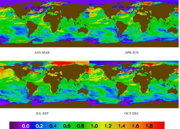
Figure 2.Seasonal mean sea-air DMS flux (lmol S m22 day21
) over 2008–2009. Also shown in black circles are cruise mean fluxes from Table 1. January–March (left to right): Knorr 06, January 2006; SO GasEx, March–April 2008; SOAP, February–March 2012. April–June (left to right): PHASE, May–June 2004; Knorr 11, June–July 2011 (top, yellow); SO GasEx, March–April 2008 (bottom, blue); DOGEE a, June–July 2007. July–September (left to right): BIO, July–August 2004; Knorr 07, July 2007; Knorr 11, June–July 2011; DOGEE a, June–July 2007; DOGEE b, July 2007. October–December (left to right): TAO, November 2003; VOCALS, October–November 2008.
Figure 3.Change inSST(C) using CMIP5 data over the 25 years from 2006–2011 to 2031–2036.
Figure 5.Change in log10(10 m wind speed) using CMIP5 data over the 25 years from 2006–2011 to 2031–2036.
effects on annual meanFof applying 25 years of predicted changes are shown in Figure S2 (supporting information). It can immediately be seen from supporting information Figure S2 that the effect of salinity changes is by far the smallest except very close to the coast. The effects ofSSTchanges are typically small and positive, increasing in areas where the flux is already large (Figure 1). The effects on flux ofU10changes are large and negative in most regions (due to the
model predicting decreased wind speed), although less so in polar regions. The effect ofDMSwchanges is highly variable, with localized
‘‘hot spots’’ of positive or negative change. The effect of changes in all four parameters is dominated by the effect of wind, so the net effect is generally negative with some positive ‘‘hot spots,’’ notably in the eastern Atlantic around 40N, which has increasedDMS
w(Figure 6), and
in the Sea of Okhotsk north of Japan, which has increased wind speed andDMSw(Figures 5 and 6). Applying
25 years of predicted changes inSST,U10, andDMSwaffects seasonal meanFas shown in Figures 7–9. The
effect of applying all four changes simultaneously is shown in Figure 10. The effect of salinity was generally as small in each season as the annual effect shown in supporting information Figure S2b, so this is not shown individually.
Our results suggest a decrease in global DMS flux in the 25 year scenario examined, mostly due to physical changes, i.e., reduced wind speed. It should be noted that if the surface DMS concentrations were to increase more than predicted by the CMIP5 model due to biological processes/feedbacks unaccounted for in the current model, the DMS flux would increase correspondingly.
3.3. Uncertainties and Error Propagation
Uncertainties and bias in the remote sensing data used to calculateFcould have a significant impact on the resultant DMS fluxes. Previous work on CO2fluxes [Land et al., 2013] has shown that the effect of random
errors inSSTandU10is of the order of 1% of the total uncertainty estimate in the Arctic, and a similarly small
proportion is likely for global DMS fluxes, hence this error source is neglected. To investigate the effect of possible bias in the input data sets, we followLand et al. [2013] and take the precautionary step of using
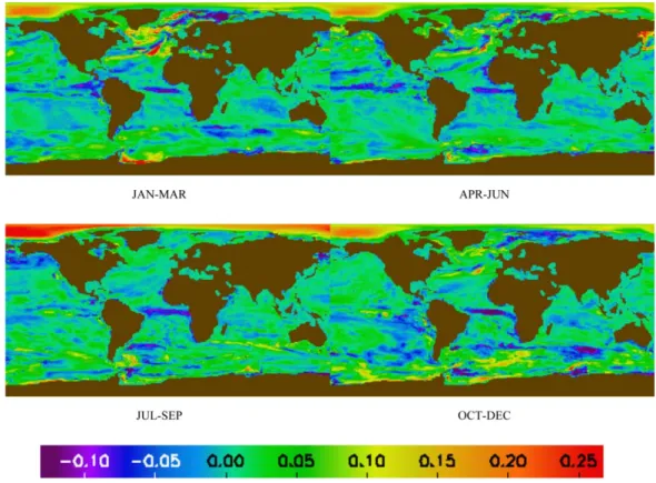
Figure 7.Changes in seasonal mean sea-air DMS flux (lmol S m22 day21
) due to 25 years of predicted changes inSST.
Table 4.Changes in Global Annual Mean DMS Flux (Tg S a21
) Due to 25 Years of Changes inSST, Salinity, 10 m Wind Speed and DMS Concentration Parameter 25 Year Change (Tg S a21
)
SST 10.46 (12.3%)
Salinity 10.10 (10.5%)
U10 24.3 (222%)
DMSw 10.33 (11.7%)
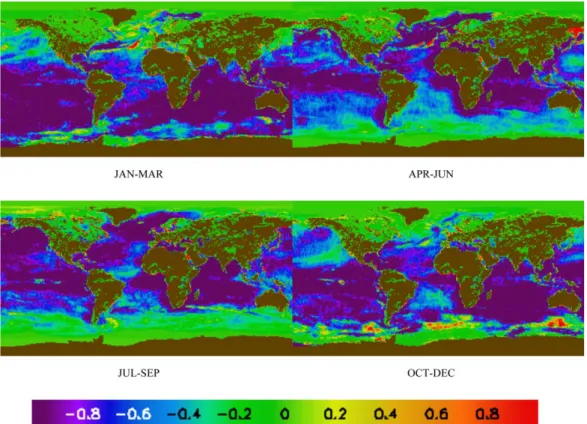
Figure 8.Changes in seasonal mean sea-air DMS flux (lmol S m22 day21
) due to 25 years of predicted changes in 10 m wind speed, on the same scale as Figure 7.
Figure 9.Changes in seasonal mean sea-air DMS flux (lmol S m22 day21
) due to 25 years of predicted changes in DMS concentration, on the same scale as Figures 7 and 8.
the square root of the sum of squares of the published global bias and standard deviation for each data set. This allows for the possibility of regional biases that cancel in the global bias but contribute to the global standard deviation. The standard deviations ofSSTandU10are 0.16C and 1.25 ms21, respectively, and the
global biases are 0.2C and 0.28 ms21, combining topffiffiffiffiffiffiffiffiffiffiffiffiffiffiffiffiffiffiffiffiffiffiffi0:16210:2250:26C andpffiffiffiffiffiffiffiffiffiffiffiffiffiffiffiffiffiffiffiffiffiffiffiffiffiffi1:25210:28251:28 ms21.
These should be considered to be upper estimates of the error due to bias. The mean and standard devia-tion ofDMSware given regionally byLana et al. [2011]. We converted these to a regional error in ln(DMSw)
and found the area weighted global average ofdln(DMSw) to be 0.12, or a 12% error inDMSw. We can use
the sensitivities found in subsection 3.2 to translate these errors inSSTandDMSwinto errors in global DMS
flux. These are 0.14 Tg S (0.7%) and 2.4 Tg S (12%), respectively. The fixed error in wind speed is incompati-ble with the proportional change used in subsection 3.2, so instead we offset all wind speeds by 1.28 ms21 and recalculated the global flux, resulting in a change in global flux of 4.8 Tg S (25%). Assuming them to be uncorrelated, these errors sum to 5.4 Tg S (27%). Correlation between errors may result in higher total errors.
Goddijn-Murphy et al. [2012] give an RMS error ofdkw55:5 660Sc
20:5
for theirkparameterization. Again assuming the worst case of bias equal to the RMS error, we recalculated fluxes using k valuesdkwgreater
than predicted, resulting in an increase in global DMS flux of 9.4Tg S (48%). Clearly this dominates the
uncertainty in global flux, which then becomes 10.9 Tg S (55%).
3.4. Contribution of Coccolithophores to the North Atlantic DMS Flux
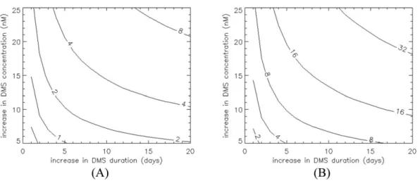
Table S1 (supporting information) shows the increase in annual mean flux over the whole North Atlantic due to DMS increases within detected coccolithophore blooms of 5, 15, and 25 nM, and with durations of 1–20 days. It is also shown as a percentage of the annual mean flux calculated from theLana et al. [2011] cli-matology. Figure 11a shows the percentage data as a contour plot, while Figure 12 shows the spatial distri-bution of the increase in flux for the most conservative case (5 nM increase for 1 day). It should be noted that the most extreme case at the upper right of Figure 11a, an increase of 25 nM for 20 days, is highly unlikely to be a good representation of North Atlantic blooms as a whole; we include these extremes to ensure that the unknown actual values are represented in supporting information Table S1 and Figures 11 Figure 10.Changes in seasonal mean sea-air DMS flux (lmol S m22
day21
) due to 25 years of predicted changes in SST, salinity, wind speed, and DMS concentration on the same scale as Figures 7–9.
and supporting information S4. For a given increase and duration, this approach is likely to be an underesti-mate of the true DMS flux as satellite backscatter cannot identify all coccolithophores (some do not shed their liths) or other DMS-producing, noncoccolithophore species. Also, it should be noted that the method ofShutler et al. [2013] specifically targets anomalously high reflectances, and so does not detect any back-ground concentration of coccolithophores, which may also contribute a DMS flux.
Our calculations suggest that the contribution to the annual DMS flux by coccolithophore blooms identified using satellite backscattering may be a relatively small proportion of theLana et al. [2011] climatological flux, which includes some contributions from coccolithophores. This suggests that noncoccolithophore spe-cies and coccolithophore spespe-cies not identifiable from space are collectively an important driver of North Atlantic seawater DMS concentrations. An alternative explanation for our analysis is that the ad hoc sam-pling approach for data in the DMS climatology has led to an inherent bias toward DMS blooms and a sub-sequent overestimate of the DMS flux. Objective sampling tracks (i.e., non bloom-focussed) for future DMS data collection would address this issue.
In summer, DMS flux from coccolithophores has the potential to be substantial (Table 2), particularly in the northeast Atlantic where blooms are more prevalent (Figure 12). To illustrate this, the increase in DMS flux due to coccolithophore blooms in the northeast quadrant of the North Atlantic (32W to 11E, 52 to 68N,
shown as a black box in Figure 12) in July is shown in Figure 11b as a percentage of the equivalent flux cal-culated from theLana et al. [2011] climatology.
The progression of coccolithophore bloom activity is illustrated in supporting information Figure S3, show-ing the distribution of bloom effect on monthly DMS flux from April to August. Blooms start in the Celtic
Sea and English Channel in April, moving to the shelf break west of Ireland in May, the shelf break north of Ireland, the North Sea and the Green-land Sea between GreenGreen-land and Iceland in June, concen-trating in a small region west of Iceland and the southern North Sea in July and August. To investigate the local impact of coccolithophore blooms, we calculated the mean percent-age effect on DMS flux for all Figure 11.(a) Change in North Atlantic annual mean flux; (b) change in monthly mean flux in the northeast Atlantic (40W–11E, 60–
68N) in July. Both are shown as a function of increase in DMS concentration within a coccolithophore bloom and duration from the last
satellite bloom detection, expressed as a percentage of the mean flux calculated from theLana et al. [2011] climatology. For reference, the annual mean flux in the North Atlantic is 4.44lmol m22
day21
and the mean flux in the northeast Atlantic in July is 10.20lmol m22 day21
. Note that these include the effects of coccolithophores.
Figure 12.Change in North Atlantic annual average DMS flux (lmol S m22 day21
) with a 5 nM increase in DMS concentration during a coccolithophore bloom and a duration of 1 day. White areas have no coccolithophore blooms detected, brown is land.
pixels with nonzero effect, i.e., pixels identified as being bloom affected (pixels not colored white or brown in Figure 12 and supporting information Figure S3). Results are shown annually in supporting information Figure S4a and for July (the month of greatest effect on North Atlantic fluxes) in supporting information Fig-ure S4b. The annual effect ranges from 1 to 38%, while the effect in July ranges from 5 to 147%.
To more accurately quantify the contribution of coccolithophore blooms to regional DMS emissions, detailed investigations are required into the relationship between bloom intensity (spectral backscattering) and seawater DMS concentration.
4. Conclusions
In this paper, we describe a new method for calculating net DMS fluxes from EO data using ak
parameterization that is calibrated for DMS, showing the applicability of EO data to the monitoring of DMS net fluxes. Specifically, we look at the effect of predicted changes in climate on the flux of DMS from ocean to atmosphere. It shows that the effect of 25 years of changes predicted by a CMIP5 climate model is globally dominated by the prediction of decreased surface wind speed, which results in a 22% decrease in global DMS flux, while changes in temperature, salinity, and DMS con-centration have smaller positive effects, with a combined effect of a 19% decrease in global flux. We also evaluate DMS emission from satellite-observed coccolithophore blooms in the North Atlantic, which is small compared to the annual climatology, but may be more important in the summertime and in the northeast Atlantic.
References
Arrigo, K. R., S. Pabi, G. L. van Dijken, and W. Maslowski (2010), Air-sea flux of CO2 in the Arctic Ocean, 1998–2003,J. Geophys. Res.,115, G04024, doi:10.1029/2009JG001224.
Balch, W. M., P. M. Holligan, S. G. Ackleson, and K. J. Voss (1991), Biological and optical properties of mesoscale coccolithophore blooms in the Gulf of Maine,Limnol. Oceanogr.,36, 629–643.
Bates, T. S., B. K. Lamb, A. Guenther, J. Dignon, and R. E. Stoiber (1992), Sulfur emissions to the atmosphere from natural sources,J. Atmos. Chem.,14, 315–337, doi:10.1007/BF00115242.
Bell, T. G., W. De Bruyn, S. D. Miller, B. Ward, K. Christensen, and E. S. Saltzman (2013), Air/sea DMS gas transfer in the North Atlantic: Evi-dence for limited interfacial gas exchange at high wind speed,Atmos. Chem. Phys. Discuss.,13(5), 13,285–13,322, doi:10.5194/acpd-13-13285-2013.
Blomquist, B. W., C. W. Fairall, B. J. Huebert, D. J. Kieber, and G. R. Westby (2006), DMS sea-air transfer velocity: Direct measurements by eddy covariance and parameterization based on the NOAA/COARE gas transfer model,Geophys. Res. Lett.,33, L07601, doi:10.1029/ 2006GL025735.
Boucher, O., and U. Lohmann (1995), The sulfate-CCN-cloud albedo effect,Tellus Ser. B,47(3), 281–300, doi:10.1034/j.1600-0889.47.issue3.1.x.
Boucher, O., C. Moulin, S. Belviso, O. Aumont, L. Bopp, E. Cosme, R. Von Kuhlmann, M. G. Lawrence, M. Pham, and M. S. Reddy (2003), DMS atmospheric concentrations and sulphate aerosol indirect radiative forcing: A sensitivity study to the DMS source representation and oxidation,Atmos. Chem. Phys,3, 49–65.
Boutin, J., J. Etcheto, L. Merlivat, and Y. Rangama (2002), Influence of gas exchange coefficient parameterisation on seasonal and regional variability of CO2 air-sea fluxes,Geophys. Res. Lett,29(8), 1182, doi:10.1029/2001GL013872.
Cameron-Smith, P., S. Elliott, M. Maltrud, D. Erickson, and O. Wingenter (2011), Changes in dimethyl sulfide oceanic distribution due to cli-mate change,Geophys. Res. Lett.,38, L07704, doi:10.1029/2011GL047069.
Charlson, R. J., and H. Rodhe (1982), Factors controlling the acidity of natural rainwater,Nature,295(5851), 683–685, doi:10.1038/295683a0. Charlson, R. J., J. E. Lovelock, M. O. Andreae, and S. G. Warren (1987), Oceanic phytoplankton, atmospheric sulphur, cloud,Nature,3526,
655–661, doi:10.1038/326655a0.
Clarke, A. D., S. Freitag, R. M. C. Simpson, J. G. Hudson, S. G. Howell, V. L. Brekhovskikh, T. Campos, V. N. Kapustin, and J. Zhou (2013), Free troposphere as a major source of CCN for the equatorial pacific boundary layer: Long-range transport and teleconnections,Atmos. Chem. Phys.,13, 7511–7529, doi:10.5194/acp-13-7511-2013.
Collins, W. J., N. Bellouin, M. Doutriaux-Boucher, N. Gedney, T. Hinton, C. D. Jones, S. Liddicoat, G. Martin, F. O’Connor, and J. Rae (2008), Evaluation of the HadGEM2 model,Hadley Cent. Tech. Note, 74, Met. Office Hadley Centre, Exeter, U. K.
Donlon, C. J., P. J. Minnett, C. Gentemann, T. J. Nightingale, I. J. Barton, B. Ward, and M. J. Murray (2002), Toward improved validation of sat-ellite sea surface skin temperature measurements for climate research,J. Clim.,15(4), 353–369, doi:10.1175/1520-0442(2002)015<0353: TIVOSS>2.0.CO;2.
Donlon, C. J., I. Robinson, K. S. Casey, J. Vazquez-Cuervo, E. Armstrong, O. Arino, C. Gentemann, D. May, P. LeBorgne, and J. Piolle (2007), The global ocean data assimilation experiment high-resolution sea surface temperature pilot project,Bull. Am. Meteorol. Soc,88(8), 1197–1213, doi:10.1175/BAMS-88-8-1197.
Donlon, C. J., M. Martin, J. Stark, J. Roberts-Jones, E. Fiedler, and W. Wimmer (2011), The operational sea surface temperature and sea ice analysis (OSTIA) system,Remote Sens. Environ,116, 140–158, doi:10.1016/j.rse.2010.10.017.
Elliott, S. (2009), Dependence of DMS global sea-air flux distribution on transfer velocity and concentration field type,J. Geophys. Res.,114, G02001, doi:10.1029/2008JG000710.
Else, B. G. T., T. N. Papakyriakou, M. A. Granskog, and J. J. Yackel (2008), Observations of sea surface fCO2 distributions and estimated air-sea CO2 fluxes in the Hudson Bay region (Canada) during the open water air-season,J. Geophys. Res,113, C08026, doi:10.1029/ 2005JG000031.
Acknowledgments
The data for this paper are available from Peter Land, [email protected]. This work was supported by seed funding from Plymouth Marine Laboratory. All Earth observation data processing was achieved using resources kindly provided by the UK NERC Observation Data Acquisition and Analysis Service (NEODAAS). M. Yang and T. Bell thank B. Huebert (U. Hawaii) and E. Saltzman (U. California Irvine) for making their in situ DMS flux data available.
Else, B. G. T., T. N. Papakyriakou, R. J. Galley, W. M. Drennan, L. A. Miller, and H. Thomas (2011), Wintertime CO2 fluxes in an Arctic polynya using eddy covariance: Evidence for enhanced air-sea gas transfer during ice formation,J. Geophys. Res.,116, C00G03, doi:10.1029/2010JC006760. Galı, M., R. Simo, M. Vila-Costa, C. Ruiz-Gonzalez, J. M. Gasol, and P. Matrai (2013), Diel patterns of oceanic dimethylsulfide (DMS) cycling:
Microbial and physical drivers,Global Biogeochem. Cycles,27, 620–636, doi:10.1002/gbc.20047.
Goddijn-Murphy, L. M., D. K. Woolf, and C. Marandino (2012), Space-based retrievals of air-sea gas transfer velocities using altimeters; cali-bration for dimethyl sulfide,J. Geophys. Res,117, C08028, doi:10.1029/2011JC007535.
Gondwe, M., W. Klaassen, W. Gieskes, and H. de Baar (2001), Negligible direct radiative forcing of basin-scale climate by coccolithophore blooms,Geophys. Res. Lett.,28(20), 3911–3914, doi:10.1029/2001gl012989.
Gunson, J. R., S. A. Spall, T. R. Anderson, A. Jones, I. J. Totterdell, and M. J. Woodage (2006), Climate sensitivity to ocean dimethylsulphide emissions,Geophys. Res. Lett.,33, L07701, doi:10.1029/2005GL024982.
Halloran, P. R., T. G. Bell, and I. J. Totterdell (2010), Can we trust empirical marine DMS parameterisations within projections of future cli-mate?,Biogeosciences,7(5), 1645–1656, doi:10.5194/bg-7-1645-2010.
Huebert, B. J., B. W. Blomquist, J. E. Hare, C. W. Fairall, J. E. Johnson, and T. S. Bates (2004), Measurement of the sea-air DMS flux and transfer velocity using eddy correlation,Geophys. Res. Lett.,31, L23113, doi:10.1029/2004GL021567.
Huebert, B. J., B. W. Blomquist, M. X. Yang, S. D. Archer, P. D. Nightingale, M. J. Yelland, J. Stephens, R. W. Pascal, and B. I. Moat (2010), Line-arity of DMS transfer coefficient with both friction velocity and wind speed in the moderate wind speed range,Geophys. Res. Lett.,37, L01605, doi:10.1029/2009GL041203.
Johnson, M. T. (2010), A numerical scheme to calculate temperature and salinity dependent air-water transfer velocities for any gas,Ocean Sci.,6(4), 913–932, doi:10.5194/os-6-913-2010.
Keller, M. D., W. K. Bellows, and R. R. L. Guillard (1989), Dimethyl sulfide production in marine phytoplankton, inBiogenic Sulfur in the Envi-ronment, vol. 393, edited by E. S. Saltzman and W. J. Cooper, pp. 167–182, AGU, Washington, D. C.
Kettle, A. J., and M. O. Andreae (2000), Flux of dimethylsulfide from the oceans: A comparison of updated data sets and flux models,J. Geo-phys. Res.,105(D22), 26,793–26,808, doi:10.1029/2000JD900252.
Lana, A., T. G. Bell, R. Simo, S. M. Vallina, J. Ballabrera-Poy, A. J. Kettle, J. Dachs, L. Bopp, E. S. Saltzman, and J. Stefels (2011), An updated cli-matology of surface dimethlysulfide concentrations and emission fluxes in the global ocean,Global Biogeochem. Cycles,25, GB1004, doi:10.1029/2010GB003850.
Land, P. E., J. D. Shutler, R. D. Cowling, D. K. Woolf, P. Walker, H. S. Findlay, R. C. Upstill-Goddard, and C. J. Donlon (2013), Climate change impacts on sea-air fluxes of CO2 in three Arctic seas: A sensitivity study using Earth observation,Biogeosciences,10(12), 8109–8128, doi: 10.5194/bg-10-8109-2013.
Liss, P. S., and P. G. Slater (1974), Flux of gases across the air-sea interface,Nature,247, 181–184, doi:10.1038/247181a0.
Malin, G., S. Turner, P. Liss, P. Holligan, and D. Harbour (1993), Dimethylsulphide and dimethylsulphoniopropionate in the Northeast Atlan-tic during the summer coccolithophore bloom,Deep Sea Res., Part I,40(7), 1487–1508, doi:10.1016/0967-0637(93)90125-M.
Marandino, C. A., W. J. De Bruyn, S. D. Miller, and E. S. Saltzman (2007), Eddy correlation measurements of the air/sea flux of dimethylsulfide over the North Pacific Ocean,J. Geophys. Res.,112, D03301, doi:10.1029/2006JD007293.
Marandino, C. A., W. J. De Bruyn, S. D. Miller, and E. S. Saltzman (2008), DMS air/sea flux and gas transfer coefficients from the North Atlantic summertime coccolithophore bloom,Geophys. Res. Lett.,35, L23812, doi:10.1029/2008GL036370.
Marandino, C. A., W. J. De Bruyn, S. D. Miller, and E. S. Saltzman (2009), Open ocean DMS air/sea fluxes over the eastern South Pacific Ocean,Atmos. Chem. Phys.,9(2), 345–356, doi:10.5194/acp-9-345-2009.
Matrai, P. A., and M. D. Keller (1993), Dimethylsulfide in a large-scale coccolithophore bloom in the Gulf of Maine,Cont. Shelf Res.,13(8), 831–843, doi:10.1016/0278-4343(93)90012-M.
Nightingale, P. D., G. Malin, C. S. Law, A. J. Watson, P. S. Liss, M. I. Liddicoat, J. Boutin, and R. C. Upstill-Goddard (2000), In situ evaluation of air-sea gas exchange parameterizations using novel conservative and volatile tracers,Global Biogeochem. Cycles,14(1), 373–387, doi: 10.1029/1999GB900091.
O’Carroll, A. G., J. R. Eyre, and R. W. Saunders (2008), Three-way error analysis between AATSR, AMSR-E, and in situ sea surface temperature observations,J. Atmos. Oceanic Technol,25(7), 1197–1207, doi:10.1175/2007JTECHO542.1.
Paasche, E. (2001), A review of the coccolithophorid Emiliania huxleyi (Prymnesiophyceae), with particular reference to growth, coccolith formation, and calcification-photosynthesis interactions,Phycologia,40(6), 503–529, doi:10.2216/i0031-8884-40-6-503.1.
Queffeulou, P., A. Benramy, and D. Croize-Fillon (2010), Analysis of seasonal wave height anomalies from satellite data over the global oceans, inESA Living Planet Symposium, edited by H. Lacoste-Francis, ESA Publ. Div., Bergen, Norway.
Quinn, P. K., and T. S. Bates (2011), The case against climate regulation via oceanic phytoplankton sulphur emissions,Nature,480(7375), 51–56, doi:10.1038/nature10580.
Shutler, J. D., M. G. Grant, P. I. Miller, E. Rushton, and K. Anderson (2010), Coccolithophore bloom detection in the north east Atlantic using SeaWiFS: Algorithm description, application and sensitivity analysis,Remote Sens. Environ.,114(5), 1008–1016, doi:10.1016/
j.rse.2009.12.024.
Shutler, J. D., P. E. Land, C. W. Brown, H. S. Findlay, C. J. Donlon, M. Medland, R. Snooke, and J. C. Blackford (2013), Coccolithophore surface distributions in the North Atlantic and their modulation of the air-sea flux of CO2 from 10 years of satellite Earth observation data, Bio-geosciences,10(4), 2699–2709, doi:10.5194/bg-10-1-2013.
Simo, R., and J. Dachs (2002), Global ocean emission of dimethylsulfide predicted from biogeophysical data,Global Biogeochem. Cycles, 16(4), 1018, doi:10.1029/2001GB001829.
Six, K. D., S. Kloster, T. Ilyina, S. D. Archer, K. Zhang, and E. Maier-Reimer (2013), Global warming amplified by reduced sulphur fluxes as a result of ocean acidification,Nat. Clim. Change,3(11), 975–978, doi:10.1038/nclimate1981.
Stark, J. D., C. Donlon, A. O’Carroll, and G. Corlett (2008), Determination of AATSR biases using the OSTIA SST analysis system and a matchup database,J. Atmos. Oceanic Technol,25(7), 1208–1217, doi:10.1175/2008JTECHO560.1.
Stefels, J., M. Steinke, S. Turner, G. Malin, and S. Belviso (2007), Environmental constraints on the production and removal of the climatically active gas dimethylsulphide (DMS) and implications for ecosystem modelling,Biogeochemistry,83(1-3), 245–275, doi:10.1007/s10533-007-9091-5.
Steinke, M., G. Malin, S. W. Gibb, and P. H. Burkill (2002a), Vertical and temporal variability of DMSP lyase activity in a coccolithophorid bloom in the northern North Sea,Deep Sea Res., Part II,49(15), 3001–3016, doi:10.1016/S0967-0645(02)00068-1.
Steinke, M., G. Malin, S. D. Archer, P. H. Burkill, and P. S. Liss (2002b), DMS production in a coccolithophorid bloom: Evidence for the impor-tance of dinoflagellate DMSP lyases,Aquat. Microb. Ecol.,26, 259–270, doi:10.3354/ame026259.
Takahashi, T., et al. (2009), Climatological mean and decadal change in surface ocean pCO2, and net sea-air CO2 flux over the global oceans,Deep-Sea Res., Part II,56(8-10), 554–577, doi:10.1016/j.dsr2.2008.12.009.
Taylor, K. E., R. J. Stouffer, and G. A. Meehl (2012), An overview of CMIP5 and the experiment design,Bull. Am. Meteorol. Soc.,93(4), 485, doi: 10.1175/BAMS-D-11-00094.1.
Twomey, S. (1991), Aerosols, clouds and radiation,Atmos. Environ.. Part A,25(11), 2435–2442, doi:10.1016/0960-1686(91)90159-5. Woodhouse, M. T., K. S. Carslaw, G. W. Mann, S. M. Vallina, M. Vogt, P. R. Halloran, and O. Boucher (2010), Low sensitivity of cloud
condensa-tion nuclei to changes in the sea-air flux of dimethyl-sulphide,Atmos. Chem. Phys.,10(16), 7545–7559, doi:10.5194/acp-10-7545-2010. Woodhouse, M. T., G. W. Mann, K. S. Carslaw, and O. Boucher (2013), Sensitivity of cloud condensation nuclei to regional changes in
dimethyl-sulphide emissions,Atmos. Chem. Phys,13, 2723–2733, doi:10.5194/acp-13-2723-2013.
Woolf, D. K., I. S. Leifer, P. D. Nightingale, T. S. Rhee, P. Bowyer, G. Caulliez, G. De Leeuw, S. E. Larsen, M. Liddicoat, and J. Baker (2007), Mod-elling of bubble-mediated gas transfer: Fundamental principles and a laboratory test,J. Mar. Syst,66(1-4), 71–91, doi:10.1016/ j.jmarsys.2006.02.011.
Yang, M., B. W. Blomquist, and B. J. Huebert (2009), Constraining the concentration of the hydroxyl radical in a stratocumulus-topped marine boundary layer from sea-to-air eddy covariance flux measurements of dimethylsulfide,Atmos. Chem. Phys.,9(23), 9225–9236, doi:10.5194/acp-9-9225-2009.
Yang, M., B. W. Blomquist, C. W. Fairall, S. D. Archer, and B. J. Huebert (2011a), Air-sea exchange of dimethylsulfide in the Southern Ocean: Measurements from SO GasEx compared to temperate and tropical regions,J. Geophys. Res,116, C00F05, doi:10.1029/2010JC006526. Yang, M., B. J. Huebert, B. W. Blomquist, S. G. Howell, L. M. Shank, C. S. McNaughton, A. D. Clarke, L. N. Hawkins, L. M. Russell, and D. S.
Covert (2011b), Atmospheric sulfur cycling in the southeastern Pacific-longitudinal distribution, vertical profile, and diel variability observed during VOCALS-REx,Atmos. Chem. Phys,11(10), 5079–5097, doi:10.5194/acp-11-5079-2011.