EXPLAINING VARIANCE IN REPRODUCTIVE SUCCESS AND FOOD SHARING IN UST’-AVAM

(1)

AND FOOD SHARING IN UST’-AVAM

by

Joellie Rasmussen

A thesis

submitted in partial fulfillment of the requirements for the degree of

Master of Arts in Anthropology Boise State University

(2)

(3)

DEFENSE COMMITTEE AND FINAL READING APPROVALS

of the thesis submitted by

Joellie Rasmussen

Thesis Title: Explaining Variance in Reproductive Success and Food Sharing in Ust’-Avam

Date of Final Oral Examination: 14 March 2014

The following individuals read and discussed the thesis submitted by student Joellie Rasmussen, and they evaluated her presentation and response to questions during the final oral examination. They found that the student passed the final oral examination. John P. Ziker, Ph.D. Chair, Supervisory Committee

David A. Nolin, Ph.D. Member, Supervisory Committee Kathryn Demps, Ph.D. Member, Supervisory Committee

(4)

This thesis is dedicated to Grandpa Jon—I know you’d be proud of me. And to Wren, who was my inspiration.

(5)

I would like to thank Dr. Ziker for the opportunity to use the research he

diligently collected, and is allowing me to prosper in terms of opportunity from his hard work. I would also like to thank Dr. Nolin for his statistical expertise and encouragement. I also thank Dr. Demps and Dr. Plew. Seeking a Master’s degree in Boise would not have been possible without the support of my family.

(6)

In light of somatic and reproductive tradeoffs modeled in evolutionary theory, this thesis conducts two analyses of men’s behavior in the indigenous hunter-gatherer

community of Ust’-Avam, northern Russia. First, a food-distribution network of men’s hunting documented in 2001 and 2003 is analyzed considering evolutionary models of food sharing: kin selection, reciprocal altruism, generosity signaling, and costly signaling. The frequency of inter-household food transfers from 36 donor households to 102

recipient households are examined using matrix regression with independent variables representing embodied, material, and relational wealth. This analysis does not support the costly signaling model, but provides robust evidence for kinship, reciprocity, and

generosity. Alongside evidence of hunter’s unidirectional food transfers to kin, hunters share reciprocally with kin and other highly skilled hunters. Furthermore, hunters appear to be sharing with the needy, rather than accumulating wealth, additional wives, or allies. Male fertility patterns of 272 Ust’-Avam men were analyzed using the same embodied, material, and relational wealth variables. Hunter skill (embodied) and hunter wealth (material) are found to be the strongest predictors of men’s age-adjusted reproductive success and age at first birth. Cash income, educational level, and number of close kin do not significantly predict men’s reproduction. Hunter production appears to be invested in their wives and existing offspring. Thus, the first analysis illustrates kin selection,

reciprocity (kin irrespective of productive ability and non-kin with high cumulative producer capacity), and generosity. The second analysis illustrates male parental

(7)

community and few wage labor opportunities for men, food production and distribution patterns are highly prosocial, and the behavior of men who are skilled and outfitted hunters appears also to provide some reproductive advantage.

(8)

DEDICATION ... iv

ACKNOWLEDGEMENTS ... v

ABSTRACT ... vi

LIST OF TABLES ... x

LIST OF FIGURES ... xi

LIST OF ABBREVIATIONS ... xii

CHAPTER ONE: INTRODUCTION ... 1

Theoretical Background ... 1

Food Sharing ... 3

Ethnographic Background ... 7

Geography ... 8

History... 9

Ust’-Avam... 10

CHAPTER TWO: RECIPROCITY, KINSHIP, SKILL, AND GENEROSITY EXPLAIN INTER-HOUSEHOLD FOOD TRANSFERS IN A SIBERIAN HUNTER-GATHERER COMMUNITY ... 12

Methods... 12

Dependent Variable ... 13

Independent Variables ... 14

Procedure ... 19

(9)

Conclusions ... 25

CHAPTER THREE: MALE REPRODUCTIVE SUCCESS AND FORMS OF WEALTH IN NORTHERN SIBERIA ... 28

Methods... 29

Dependent Variables ... 29

Independent Variables ... 30

Results ... 30

Age-Adjusted Reproductive Success ... 30

Age at First Birth ... 36

Conclusions ... 42

CHAPTER FOUR: DISCUSSION AND CONCLUSION... 44

Food Sharing: Models of Multiplicity ... 44

Reproductive Success and Wealth ... 52

Conclusion ... 55

REFERENCES ... 57

(10)

Table 2.1 Example of matrix used for frequency of transfers ... 14

Table 2.2 Individually entered variables predicting frequency of transfers ... 20

Table 2.3 Main effects model predicting frequency of transfers ... 21

Table 2.4 Main effects and interaction terms model predicting frequency of transfers ... 22

Table 2.5 Final model predicting frequency of transfers ... 23

Table 2.6 Model exploring the possible effects of reciprocity in other currencies in predicting frequency of transfers ... 24

Table 3.1 Age-adjusted RS: Embodied variables - individually entered ... 31

Table 3.2 Age-adjusted RS: Material variables - individually entered ... 33

Table 3.3 Age-adjusted RS: Relational variables - individually entered ... 35

Table 3.4 Age-adjusted RS: Final model ... 36

Table 3.5 Age at first birth: Embodied variables - individually entered ... 37

Table 3.6 Age at first birth: Material variables - individually entered ... 39

Table 3.7 Age at first birth: Relational variables - individually entered ... 41

Table 3.8 Age at first birth: Final model ... 42

(11)

Figure 1. Map of Ust Avam... 9 Figure 2. Fictitious diagram illustrating coefficients of relatedness between

members of two households. The maximum relatedness is r = 0.5, whereas the average would be r = 0.1875. ... 15 Figure 3. Linear regression plot: hunter skill evaluations ... 32 Figure 4. Linear regression plot: hunter material wealth ... 34 Figure 5. Kaplan-Meier plot of likelihood of age at first birth by hunter skill

evaluations ... 38 Figure 6. Kaplan-Meier plot of age at first birth by hunter material wealth ... 40

(12)

RS Reproductive Success

MRQAP Multiple Regression Quadratic Assignment Procedure

HBE Human Behavioral Ecology

(13)

CHAPTER ONE: INTRODUCTION

Theoretical Background

Many anthropologists look to hunting and gathering societies to provide insights into the behaviors of human ancestors. Knowing that all humans had hunting-and-gathering economies prior to the development of other means of subsistence allows anthropologists to examine modern day hunter-gatherer societies in hopes of explaining the evolution of certain human traits. One of these traits is food sharing. In this thesis, I examine the hypotheses of food sharing as mechanisms for the evolution of cooperation and test data collected from Ust’-Avam male hunters. As many anthropologists have asked in other study areas, I ask why hunters in this community share food. What predicts these food transfers? How do these results support food sharing hypotheses? The findings from the results of the following analyses contribute to a larger debate, which seeks to answer why humans share food and how food-sharing evolved. Food-sharing is a

cooperative behavior, and outside of provisioning, it seems to be a behavior at odds with natural selection. Food sharing is a universal human trait, and is found ubiquitously in hunter-gatherer societies, leading to evidence that the trait was selected for.

(14)

does with the food he decides to keep. Does he invest this meat into gaining access to new mates, investing it in potential offspring with other women? Or does he invest his resources into his current mate and offspring? Furthermore, how does his wealth and skill affect these decisions?

A hunter deciding whether to invest his resources into gaining access to additional mates or investing them in his current mate and offspring is an example of a tradeoff. These two choices are not mutually exclusive. A hunter is likely to distribute some of the meat or fish he acquired, and keep the rest. A hunter may also spend more time acquiring knowledge, skills, and material wealth, and, in doing so, foregoes investing this time and his resources in producing offspring. Rather than invest his resources in current offspring, he is choosing to invest his resources in future offspring.

Borgerhoff-Mulder (2000) examines life history traits as tradeoffs of quantity-quality of offspring and current versus future reproduction decisions among the Kipsigis. Borgerhoff-Mulder found the women among the Kipsigis were producing an optimal number of children, but the men were producing a suboptimal number of offspring. Women were making decisions in the quantity-quality tradeoff of offspring that lead to them gaining optimal fitness. They were more likely to increase fitness gains across generations by having fewer children and enhancing their quality. In order to gain optimal fitness, the men were more inclined to have more children, and were more interested in investing in reproductive efforts.

(15)

example of the reproductive-versus-parenting tradeoff. Rather than invest the meat they catch in gaining potential access to additional mates by sharing the food with individuals outside of the household, they choose instead to provision their current spouse. Another explanation for this correlation is dyadic reciprocity, where hunter’s exchange meat for direct access for mates. Indirect reciprocity is delayed and comes from multiple

individuals, usually in the form of reputation building. Costly signaling acts on the hunter using his hunting skill to broadcast the signal that he is a superior mate.

Food Sharing

Food sharing occurs universally among hunter-gatherers and the study of this behavioral trait opens a window for researchers to understand the evolution of cooperation. Although primate species do participate in food sharing outside of

(16)

altruism, costly signaling and tolerated scrounging. These four have been subject to much debate in the last two decades in human behavioral ecology.

Kin Selection

Kin selection is often proposed as an explanation for altruistic or cooperative behavior. Natural selection supports strategies that favor the success of kin, and possibly at the cost of the individual’s own reproductive success. Individuals are expected to share with kin above non-kin. Hamilton’s rule (1964) states that only when the benefit (B) gained and relatedness factor (r) between the two individualscombined outweigh the cost (C) of the action will a transfer occur (C < B*r). The general premise of kin selection is that because kin share some genes, fitness might be gained by an individual when its kin reproduce, even if the individual does not. Therefore, altruistic acts benefiting one’s kin might indirectly benefit oneself, in terms of fitness. Two related individuals, for example, siblings. have the probability of sharing 50% of their alleles. If one individual incurs a cost that might inhibit their reproductive success, but benefits their siblings’ reproductive success, there is a likelihood the trait that prompted the first sibling would also exist in, and be passed down through, the second individual. In other words, altruistic traits may be selected through the benefit to kin. Kin selection in food-sharing proposes that individuals will be more willing to share with those who are more closely related by Wright’s coefficient of relatedness r (Kaplan and Gurven, 2001).

Reciprocal Altruism

(17)

behaviors might evolve among unrelated individuals. He uses the example of a drowning man. There is little incentive to save the man, especially with potentially great cost (such as death, in this case). So why would someone choose to save the man? If an individual is at as much of risk of drowning in the future, and the risks of drowning can be mitigated by being saved by another individual, then altruism might be selected for.

Reciprocal altruism in food sharing requires that the donor bears a cost that benefits another, and that the recipient of the altruistic act receives a benefit that is higher than the costs. Food shared reciprocally should be contingent on previous transfers. Reciprocal altruism is more likely to occur when food procured is in large, asynchronous packages (Kaplan and Hill, 1985), based on the law of diminishing returns. The first portion an individual acquires is of more value than the second portion, which is of more value to the individual than the third, and this continues on for every subsequent portion. A large package is composed of many portions, so when an individual has consumed their third portion of the package, the value of the fourth, unconsumed portion is greater to another individual, because it is their first portion. The portion is of less value to the individual who acquired the packaged than it is to the individual who hasn’t consumed any portions. The individual performing the altruistic behavior must receive a benefit from the original recipient of the altruistic act in order for cooperation to evolve via this evolutionary mechanism.

(18)

basic Prisoner’s Dilemma is a game constructed around a two-by-two matrix. Two players may choose to cooperate and receive a benefit, or cheat and secure an even greater benefit while imposing a cost on the other. However, if both individuals cheat, then they both incur a cost. The tit-for-tat strategy involves going into a situation like the Prisoner’s Dilemma with good faith by cooperating on the first move, and then copying the other player’s behavior for every subsequent move. This strategy is based in

reciprocity.

Costly Signaling

(19)

Tolerated Scrounging

Tolerated scrounging has been proposed as an alternative to kin selection and reciprocal altruism. Tolerated scrounging is a simpler theory, and occurs when an individual with food realizes the cost of defending the food is greater than the cost of giving it up to encroachers. Generally, as the marginal value of a food package decreases to the hunter, the more likely they are to give up portions of food to those who ask or demand (Blurton Jones, 1987). Tolerated scrounging is expected to occur with large, asynchronous packages. Again, if the individual who procured the package has consumed the first (or more) portion of the package, the second portion is of less value to that individual, but may be of greater value to another, second individual. If the second individual pressures the first to give up a portion of the package, the value of that portion may be low enough that the first individual decides defending the portion is too great. The second individual may realize the value of the first portion is great enough to initiate conflict/other costs on the first individual. The costs imposed on the hunter can be

physical (through violence) or social.

Ethnographic Background

(20)

Geography

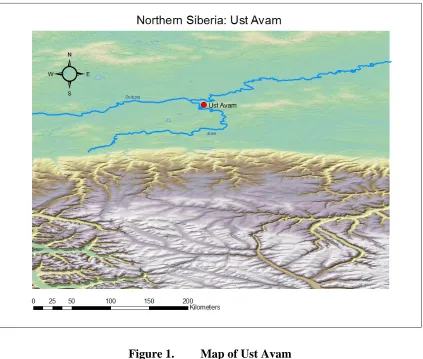
Located in the Taimyr region of central Siberia, Ust’-Avam lies at 71° North latitude. The village is located along the Avam River, at 71° 07’ N and 92° 49’ E, on the Taimyr Peninsula in Central Siberia. The Avam River flows out of the Putoran Plateau north into the Dudypta River, shown on Figure 1, which then flows into the Piasina River. The winters are long and cold, and the summers are short and mild (Ziker, 2002). Ziker writes the area is in close proximity to a forest of Daur’s larch, which extends across the lowlands and surrounds the village. There are multiple lakes in the area.

(21)

Figure 1. Map of Ust Avam

The village’s remoteness inflates travel costs, making it difficult to travel to or from the community. Travel is either by helicopter, boat, or snowmobile. The Dudpyta and Avam Rivers act as the main source of travel in the summer.

History

(22)

had collectivized most of the domestic reindeer. In 1971, the community of Ust’-Avam was created. Ust’-Avam sat on ten million hectares set aside to create a new

administrative hunting district, “Taimyrskii,” which focused on commercial hunting, trapping, and fishing. At this point, community members became fully integrated in the Soviet planned economy and were paid decent monthly salaries for a variety of jobs including staff hunter, seamstress, stove stoker, janitor, etc. Villagers received wages and pensions like all other workers in the Soviet Union. In addition, all domestic reindeer were slaughtered by 1978 and the community became fully dependent on combustion-powered transportation. Since the Dolgan and Nganasan lost much of their traditional autonomy and became dependent on outside sources of equipment, fuel, and cash, the community was very negatively affected by the collapse of the USSR. The importance of traditional subsistence activities has been emphasized with the decentralization of the Russian government since the fall of the Soviet Union (Ziker, 2002). Since the early 1990s, few jobs are salaried and those are reserved for a select few. The costs of fuel and equipment increased drastically so Ust’-Avam hunters give more emphasis to hunting and fishing for subsistence rather than commercial sales. In addition, traditional modes of hunting and gathering, such as game trapping, became more widespread.

Ust’-Avam

(23)

They also trapped and fished. Both were traditionally semi-nomadic. After the

establishment of the Government Hunting Enterprise Taimyrski alongside the permanent village in 1971, the state provided snowmobiles, rifles, and ammunition for hunting. In the 1990s and early-to-mid 2000s, as such goods became costly and most hunters were no longer receiving a wage, snowmobiles and other equipment were found to be aging and failing. Many hunters were focusing more on local prey as travel costs increased. In 1996, a few hunters were able to sell their game for cash. However, cash income remains rare.

In the growing season, women and children will collect what mushrooms and berries they can gather (Ziker, 2002). Caribou are hunted in late fall and early spring at river crossings, and during the summer, fall, and winter on land. Geese are hunted in the spring and the summer. Fishing occurs year-round, with ice-net fishing in the winter, open-water net-fishing and seine fishing in the summer, and thin-ice fishing in the spring. Arctic fox trapping occurs in the winter, but can be costly due to transportation

(24)

CHAPTER TWO: RECIPROCITY, KINSHIP, SKILL, AND GENEROSITY EXPLAIN INTER-HOUSEHOLD FOOD TRANSFERS IN A SIBERIAN

HUNTER-GATHERER COMMUNITY

In the community of Ust’-Avam, the fall of the Soviet Union decreased the amount of outside resources available to the people. An increased reliance on traditional modes of subsistence – hunting, trapping and fishing – was noted by Ziker in his visits to the area (Ziker, 2002; Ziker, 2003; Ziker and Schnegg, 2005). Food sharing is pervasive in hunter-gatherer societies, and is seen in Ust’-Avam. Hunters share the meat they hunt in the community with kin, neighbors, friends, and acquaintances. What determines with whom a hunter will share with? This chapter seeks to predict variation in inter-household sharing between donor, hunter households, and recipient households. In order to do so, several variables are examined. Household characteristics of hunting skill and material wealth, previous transfers of meat or other items and services, and inter-household relatedness to kin are all analyzed. In this chapter, I outline the methods used to conduct these analyses and their results. This outline includes descriptions of each variable and the procedures used. Finally, I summarize the conclusions these results point to.

Methods

(25)

noted by Ziker (M.S. 2013). The variables examined were collected in 1997, 2001, and 2003, and some in 2007.

Dependent Variable

What best predicts food sharing in Ust’-Avam? To answer this question, the frequency of transfers occurring between households was analyzed using several

independent variables. These transfers occurred after 77 hunting excursions involving 36 hunters. Ziker recorded the amount of meat and fish acquired, and the amounts consumed or distributed for all 77 excursions. In order to examine dyadic relationships between households, a matrix regression analysis is used. Each variable is entered into a 177x177 matrix. The 177x177 matrix consists of all pairs of households in the community, with donor households represented by row and recipient households represented by column. To create the frequency of transfers matrix, the number of transfers occurring from the donor household to the recipient household is entered as the value of the matrix cell. For this example, please refer to Table 2.1. If household A gave food once to household B, the value in cell 2 would be 1. If household B never reciprocated, the value in cell 2 would be 0. Two hundred and four sharing events were analyzed between 36 donor households and 102 recipient households, though all households participated in the study. Non-hunted food sharing events were not recorded in this study, so the 36 donor

(26)

Table 2.1 Example of matrix used for frequency of transfers

A B

A [cell 1] [cell 2] 1

B [cell 3] 0 [cell 4]

Independent Variables

Maximum Genealogical Relatedness

Does kinship best predict inter-household transfers? In order to analyze the frequency of transfers with kinship, genealogical relatedness needed to be calculated for each household. For a pair of households, the genealogical relatedness for each individual in one household was determined in relation to all other individuals in the other

(27)

Figure 2. Fictitious diagram illustrating coefficients of relatedness between members of two households. The maximum relatedness is r = 0.5, whereas the

average would be r = 0.1875.

Sum of Maximum Hunter Skill

(28)

evaluator was biased towards rating hunters higher or lower than other evaluators, then the imputed ratings for that evaluator would reflect this bias consistently across all hunters. In order to check that imputing ratings were still valid, the imputed ratings were summed and, along with the summed un-imputed ratings, linearly regressed against age-adjusted reproductive success (See Chapter 3). The results were similar and justify using the larger dataset (imputed hunter skill evaluations: adj. R2 = 0.101, F1, 140 = 16.824, β =

0.328, t = 4.102, p = 0.000; non-imputed hunter skill evaluations: adj. R2 = 0.124, F1, 55 =

8.872, β = 0.374, t = 2.963, p = 0.005). The independent variables representing dyadic skill relationships use the maximum hunter skill evaluation for each household in cases where there were two or more hunters in a household. The summed values of the hunter skill evaluations of an inter-household dyad are used to create the sum of max hunter skill matrix.

Sum of Maximum Hunter Wealth

Each hunter was assigned a wealth value on a scale of 0 - 5. This value was determined by the ownership of any of the following four items in the year 2003: snowmobile, boat motor, rifle, and shotgun; and by the occupation of a hunting territory in 1997, 2003, or 2007. A Mokken scaling analysis, performed in R, was used to

determine the validity of creating a scale from these five items. A Mokken analysis is similar to a Guttman’s scaling analysis, and is used to construct and determine the

(29)

than one hunter in a household, and these values were summed in a 177x177 matrix – that is, the highest material wealth value was summed for each inter-household dyad.

Difference of Maximum Hunter Skill

The sum of maximum hunter skill evaluations variable is a matrix of the sums of hunter skill in an inter-household dyad, as discussed above. Here, instead of summing the two hunter skill evaluations in a household pair, a matrix was constructed by finding the difference between the skill evaluations of each pair of households. The recipient skill rating was subtracted from the donor skill rating. I plan to capture differences in producer ability with this variable.

Difference of Maximum Hunter Wealth

The sum of maximum hunter wealth variable is a matrix of the sums of the material wealth ratings in an inter-household dyad, as I discussed previously. In order to measure differences in wealth, the differences (as opposed to the sums) of the ratings between households are found and entered into a matrix. The recipient hunter wealth scale was subtracted from the donor hunter wealth scale. I plan to capture differences in hunting reputation with this variable.

Frequency of Transfers Transposed

(30)

household B. If the matrix is transposed, the value for cell 2 is 0, because B never gave to household A. The value for cell 3 becomes 1. The other two cells remain undefined. When frequency of transfers is regressed with frequency of transfers transposed as the independent variable, results indicate the level of reciprocity occurring in inter-household transfers, that is, the correlation of B’s giving to A with A’s giving to B.

Frequency of Receiving

Each sharing event that occurred from the 77 hunts in field visits by Ziker in 2001 and 2003 was coded into two separate dummy variables, obligatory sharing and voluntary sharing. The interviewee (donor) was asked three questions.

1) Why did you share?

2) What did you get out of sharing?

3) Did the recipient ever give you bush food or anything else?

If the answers indicated that the interviewee felt obligated to give meat or fish in some way, then the obligatory variable was coded with a 1. If the interviewee did not feel obligated to give food, then the obligatory variable was coded with a 0. If the interviewee had voluntarily shared and felt no expectation to share, the voluntary variable was coded with a 1. If the sharing event indicated the interviewee had shared because he felt

(31)

him a rifle or boat motor), and for the second case, indicating that the recipient had given to the hunter something the hunter would not feel obligated to reciprocate (for example, tea). These two matrices were summed, indicating any sort of sharing with the hunter prior to the hunt that may have occurred in a different ‘currency.’

Procedure

Multiple-Regression Quadratic Assignment Procedure (MRQAP) performed by UCINET 6.0 was used to analyze these matrices. QAP is used in cases where the data violate the assumption of independence (Krackhardt, 1988). The QAP ‘scrambles’ the dependent matrix by using the same permutation for rows and for columns. Several hundred permutations of the dependent matrix result in a sampling distribution to use as the null hypothesis. The original dependent matrix and the permuted matrix are both regressed with the independent matrix.

If the regression coefficients (or R2) from the original matrix are in the extreme percentile of the distribution of coefficients (or R2) produced by the permuted matrices, the null hypothesis can be rejected.

Results

(32)

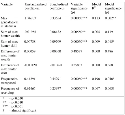
(β = 0.25977, p = 0.00050) are significant as variables. The frequency of receiving variable when individually entered is not significant, although it approaches significance. So, while frequency of receiving may have a significant effect on the frequency of transfers, the variance it explains is not large enough to be significant at the model level.

Table 2.2 Individually entered variables predicting frequency of transfers

Variable Unstandardized coefficient Standardized coefficient Variable significance (p) Model R2 Model significance (p) Max genealogical relatedness

1.76707 0.33654 0.00050*** 0.113 0.002**

Sum of max hunter wealth

0.01955 0.06432 0.00550** 0.004 0.119

Sum of max hunter skill

0.00738 0.09709 0.00050*** 0.009 0.015* Difference of

max hunter wealth

0.00059 0.00360 0.48577 0.000 0.486

Difference of max hunter skill

-0.00120 -0.01498 0.25837 0.000 0.368

Frequencies transposed

0.44291 0.44291 0.00050*** 0.196 0.046* Frequency of

receiving

0.92465 0.25977 0.00050*** 0.067 0.063† * = p<0.050

** = p<0.010 *** = p<0.001

† = almost significant

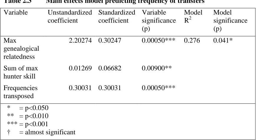
Table 2.2 shows the results of entering the three main effects, determined from the individually entered variables, to predict the frequency of transfers. The three

(33)

frequencies transposed (which represents reciprocity). When entered together, each variable remains significant. The model is significant, and the R2 is 0.276, resulting in almost 28% of the variance in frequency of transfers explained by these three variables.

Table 2.3 Main effects model predicting frequency of transfers

2.20274 0.30247 0.00050*** 0.276 0.041*

0.01269 0.06682 0.00900** Frequencies

transposed

0.30031 0.30031 0.00050*** * = p<0.050

** = p<0.010 *** = p<0.001

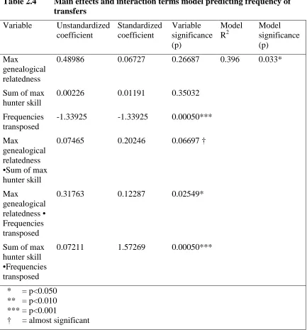
Is there any variance that is not explained by these variables individually, but might be explained by some interaction of these variables? In order to answer this question, three interaction terms were created. The first, max genealogical relatedness • sum of max hunter skill, was created by multiplying the corresponding cell values of these two matrices. The second, created in the same way as the first, was max

(34)

sum of max hunter skill, are no longer significant. Furthermore, the sign on the

coefficient of frequencies transposed has moved from positive to negative (β = -1.33925,

p = 0.00050), indicating an increase in sharing with households who do not reciprocate, after controlling for a propensity to share with relatives and other skilled hunters who reciprocate. It is important to note that the max genealogical relatedness • sum of max hunter skill variable approaches significance (β = 0.20246, p = 0.06697).

Table 2.4 Main effects and interaction terms model predicting frequency of

transfers

0.48986 0.06727 0.26687 0.396 0.033*

0.00226 0.01191 0.35032

-1.33925 -1.33925 0.00050*** Max

genealogical relatedness •Sum of max hunter skill

0.07465 0.20246 0.06697 †

Max

genealogical relatedness • Frequencies transposed

0.31763 0.12287 0.02549*

Sum of max hunter skill •Frequencies transposed

0.07211 1.57269 0.00050***

* = p<0.050 ** = p<0.010 *** = p<0.001

(35)

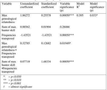
Is there a more parsimonious model? The decision to remove the interaction term max genealogical relatedness •sum of max hunter skill only slightly affected the overall R2 of the model, and did not affect its significance. Of some interest is that max

genealogical relatedness is again significant in the final model (β = 0.25578, p =0.00050). It is important to note here that the sign on the coefficient of frequencies transposed remains negative.

Table 2.5 Final model predicting frequency of transfers

1.86272 0.25578 0.00050*** 0.395 0.033*

0.00362 0.01904 0.28486

-1.43521 -1.43521 0.00050*** Max

0.32785 0.12682 0.01949*

Sum of max hunter skill •Frequencies transposed

0.07718 1.68334 0.00050***

* = p<0.050 ** = p<0.010 *** = p<0.001

† = almost significant

(36)

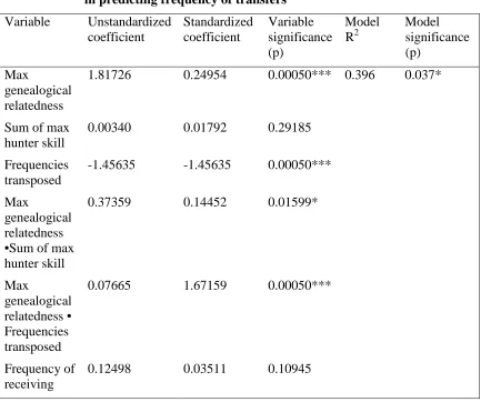
that this variable is significant when individually entered to predict the frequency of transfers. The results in Table 2.5 indicate that the frequency of receiving is not a significant predictor of the frequency of transfers in this exploratory model, indicating that most of the variance explained by this variable is also explained by other variables. The model R2 remains mostly unchanged (though the significance of the model does slightly increase (p = 0.037)). When combined with other variables, possibly frequencies transposed, frequency of receiving does not predict frequency of transfers, indicating that reciprocity does not occur in other currencies significantly enough to predict food

transfers.

Table 2.6 Model exploring the possible effects of reciprocity in other currencies

in predicting frequency of transfers

1.81726 0.24954 0.00050*** 0.396 0.037*

0.00340 0.01792 0.29185

-1.45635 -1.45635 0.00050*** Max

genealogical relatedness •Sum of max hunter skill

0.37359 0.14452 0.01599*

Max

0.07665 1.67159 0.00050***

Frequency of receiving

(37)

* = p<0.050 ** = p<0.010 *** = p<0.001

Conclusions

The best model to predict variations in food transfer frequencies includes kinship, reciprocity, and household hunting skill. Hunting skill only predicts transfers when included with other variables controlling for the interaction terms, and is not significant. The results from the final model support this conclusion, and also show that this variation is not explained by these three variables alone, but also relies on an amount of interaction between hunter skill and reciprocity, and kinship and reciprocity. This final model, which includes the main effects and these two interaction terms, explains almost 40% of the variance in inter-household food transfers. Aside from the findings of this final model, the results show several other conclusions.

First, the model (Figure 2.5) shows transfers increase in frequency as

inter-household relatedness increases, with a standard coefficient (β) of 0.25578 (p = 0.00050), controlling for reciprocity, skill, and interaction terms. This result supports the kin

provisioning hypothesis discussed in Chapter 1. Second, increases in frequency of transfers, when controlled for kinship and skill and the interaction terms, result in significant decreases in reciprocal transfers, showing a shift from contingency to

(38)

receiving variable, which was significant when entered individually to predict frequency of transfers. This indicates that reciprocity is occurring in the community in other

currencies, but the model was not significant, and the variable was not significant when added to the final model. I conclude that while reciprocity does occur in other currencies, it does not significantly predict the frequency of transfers and that these transfers are truly generous – they are not reciprocated.

Third, reciprocity occurs between highly skilled households, as noted by the significance of the interaction term sum of skills • frequency of transfers (β = 1.68334, p

= 0.00050), independent of kinship, generous transfers, and the interaction between kinship and reciprocity. Fourth, reciprocity also occurs between related households (β = 0.03560, p = 0.00050), independent of the interaction of skill and reciprocal transfers, kinship, skill, and generous transfers. Recent studies have also illustrated an interaction with kinship and reciprocity (e.g., Nolin, 2010). I will expand on these in Chapter 4.

Hunters with higher producer capacity do not give more frequently to those with lower capacities, and choose instead to share with those who are more likely to

reciprocate, as represented by the strength of the interaction term between sum of skill and frequency of transfers transposed. The variable representing the household

(39)

(40)

CHAPTER THREE: MALE REPRODUCTIVE SUCCESS AND FORMS OF WEALTH IN NORTHERN SIBERIA

Research in the community of Ust’-Avam, following the collapse of the Soviet Union, can provide insight into individuals’ decisions in an environment of change. As the members of this community move away from a commercial hunting economy towards a more traditional, subsistence economy, questions central to the HBE field are asked here. What best explains these hunters’ reproductive success? How do different types of wealth affect this success, and how well do they predict when a hunter will start his reproductive career? This section looks to answer the broader question of what men do with the resources they choose to keep in light of life-history tradeoffs concerning seeking new mates and potential future offspring, or provisioning current mates and offspring.

(41)

Methods

What best predicts variation in men’s reproductive success and when they will reproduce? The sample includes all 272 men 15 years of age and over in the Ust’-Avam community. In order to answer this question, age adjusted reproductive success (RS) and age at first birth are regressed against three classes of wealth determined by nine separate variables. These are the same three wealth classes described by Smith et al. (2010) and are material, embodied, and relational wealth. Embodied wealth includes such

intangibles as education, skills, and health. Material wealth is the ownership of physical, tangible property, and the most easily measured. The number and quality of social relations determines social capital or, as it’s called in this study, relational wealth.

Dependent Variables

What best predicts men’s reproductive success? To answer this question,

reproductive success needs to be defined and quantified. Here, reproductive success only includes children survived to age 5 at census (2007). Age is controlled for by using the residuals of the number of children survived to age 5 with age and age2 as predictors. Age is determined by age at census (2007). Age-adjusted RS is used as the dependent variable in linear regressions and using this variable serves to control for the very strong

correlation between age and reproductive success, allowing the RS of men of different ages to be compared.

(42)

age at first birth requires a hazard-function analysis rather than a linear regression, the Cox regression is a hazard-function analysis provided by SPSS.

Independent Variables

Three classes of wealth are tested in this analysis: embodied, material, and relational. Embodied wealth can often include skills, education, and health statistics such as BMI. Here, I used the education level recorded in the census, and the hunter skill evaluation scale as described in Chapter 2. The variables used to describe material wealth include the material wealth scale also described in Chapter 2, and the amount of cash income recorded in a survey conducted among a sub-sample of hunters in 1997. There are few cases for this variable. Relational wealth is generally defined with variables that act as proxy for the strength of an individual’s social network. In this case, I use the count of parents, the count of siblings, the count of parents’ siblings, and the count of parents’ siblings’ offspring. These four variables were provided from Ziker’s extensive

genealogical data updated in 2007 inputted into the program Descent (Hagen, 2005). I have included an additional measure of relational wealth in the form of a formal hunting status. Each individual was scored on a scale of 1 to 5 (staff hunter, brigade hunter, amateur, etc.) as an indicator of social relations. I have inverted this scale to use in regressions.

Results

Age-Adjusted Reproductive Success

Each of the nine variables was entered individually in both linear and Cox

(43)

Then, each variable was entered individually in a Cox regression to determine their effect on age at first birth. Each variable representing embodied wealth was individually

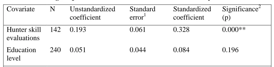
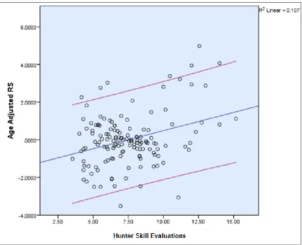
regressed against age-adjusted reproductive success using SPSS. Bootstrapping was used in order to control for known interdependence in the data, and leads to conservative t-test results. Of the two, only the hunter skill evaluations variable was significant (β = 0.328, p

= 0.000). Table 3.1 illustrates these results.

Table 3.1 Age-adjusted RS: Embodied variables - individually entered

Covariate N Unstandardized coefficient

Standard error1

Standardized coefficient

Significance2 (p)

Hunter skill evaluations

142 0.193 0.061 0.328 0.000**

Education level

240 0.051 0.044 0.084 0.196

1 Robust bootstrapped standard errors, 2 T-test significance, * Significant at p<0.05, ** Significant at p<0.01, † Approaching significance

(44)

Figure 3. Linear regression plot: hunter skill evaluations

(45)

small ‘n’ would alter the results of the final model, further justifying not including this variable.

Table 3.2 Age-adjusted RS: Material variables - individually entered

Covariate N Unstandardized coefficient

Standard error1

Standardized coefficient

Significance2 (p)

Material wealth scale

272 0.221 0.064 0.255 0.000**

Cash income

21 3.696E-006 1.9E-005 0.069 0.7666

(46)

Figure 4. Linear regression plot: hunter material wealth

(47)

approaches significance (β = -0.115, p = 0.058). While the significance of this variable does not meet the threshold set, it does border it, and the number of full cousins a hunter has might have a negative influence on the number of children he has.

Table 3.3 Age-adjusted RS: Relational variables - individually entered

Covariate N Unstandardized coefficient Standard error1 Standardized coefficient Significance2 (p) Number of siblings

272 -0.011 0.038 -0.017 0.781

Number of parents

272 -0.012 0.088 -0.007 0.903

Number of parents’ siblings

272 -0.021 0.025 -0.031 0.610

Number of parents’ siblings’ offspring

272 -0.019 0.006 -0.115 0.058†

Formal hunting status

138 0.262 0.103 0.259 0.002**

(48)

Table 3.4 Age-adjusted RS: Final model

Covariate N Unstandardized coefficient Standard error1 Standardized coefficient Significance2 (p) Hunter skill evaluations

133 0.142 0.057 0.237 0.014*

Material wealth

133 0.175 0.079 0.210 0.029*

Overall Model fit (R2) = 0.153, F-test significant, p = 0.001

Age at First Birth

In order to determine when a hunter in the community may expect to experience a first birth, a Cox regression (or Cox proportional hazards analysis) was performed. Each of the nine independent variables was entered individually against the dependent variable of age at first birth. Again, these nine variables are grouped into three categories of wealth: embodied, material, and relational. First, the relational wealth variables were individually entered in a Cox regression. The results are depicted in Table 3.5, and show that again, like in the linear regression predicting reproductive success, only hunter skill evaluations are significant when predicting age at first birth (Exp(B) = 1.091, p = 0.045). Of note here, though, is that the education level approaches significance (Exp(B) = 1.106,

(49)

influence on men’s expected age at first birth: completing 11 years of school in the community may be a general indicator of embodied capital, and thus make these men more attractive as mates. If men left the community for secondary education, they would likely experience a delay in age at first birth. In post-demographic transition economies, individuals delay reproduction to build capital. However, since there are so few

employment opportunities that require education (and these are often filled by ethnicities other than Dolgan or Nganasan), education is not as beneficial to an individual in

building wealth.

Table 3.5 Age at first birth: Embodied variables - individually entered

Covariate N B Standard

error1

Exp(B) Significance2 (p) Hunter skill

evaluations

142 0.087 0.035 1.091 0.045*

Education level 240 0.101 0.053 1.106 0.056†

1 Robust bootstrapped standard errors, 2 Wald test significance, * Significant at p<0.05, ** Significant at p<0.01, † Approaching significance

(50)

skilled. The plot indicates that highly skilled hunters (the green line) are more likely to experience a first birth by the age of 35 than those who are less skilled. Highly skilled hunters, if they are going to experience a first birth, do so by the time they are 35, whereas moderately skilled hunters will do so by the time they are 55 years old. Interestingly, this plot shows that the least skilled hunters are also the least likely to experience a first birth.

Figure 5. Kaplan-Meier plot of likelihood of age at first birth by hunter skill

(51)

Next, the material wealth variables were entered individually to predict age at first birth. Again, only the wealth scale was significant (Exp(B) = 1.148, p = 0.012), and cash income is very much not significant (Exp(B) = 1.000, p = 0.695). Since cash income is so insignificant, and again, because its n is so small (21), it is not included in determining the final model.

Table 3.6 Age at first birth: Material variables - individually entered

error1

Exp(B) Significance2 (p) Material wealth scale 272 0.138 0.046 1.148 0.012*

Cash income 21 0.000 0.000 1.000 0.695

(52)

Figure 6. Kaplan-Meier plot of age at first birth by hunter material wealth

(53)

Table 3.7 Age at first birth: Relational variables - individually entered

error1

Exp(B) Significance2 (p) Number of siblings 272 -0.089 0.050 0.915 0.106

Number of parents 272 0.059 0.161 1.061 0.704 Number of parents’

siblings

272 -0.027 0.080 0.973 0.720

272 -0.023 0.021 0.977 0.183

Formal hunting status 138 0.159 0.072 1.172 0.043*

These nine variables (excluding cash income) were entered into a final model to predict age at first birth using the backwards-stepwise procedure with the Cox regression. Of the eight variables entered, only the material wealth scale, the number of parents’ siblings, and the number of parents’ siblings’ offspring are kept in the final model. Of particular interest here, is that only the material wealth scale is significant (Exp(B) = 1.219, p = 0.004), as shown in Table 3.8. The other two relational variables are not significant in the final model, nor were they significant when individually entered. These variables seem to not negatively affect the overall model fit in, and SPSS found that their elimination did not improve the model and the variation they explain, while neither large nor significant, is unique. This may be one possible explanation for why they are

(54)

Table 3.8 Age at first birth: Final model

error1

Exp(B) Significance2 (p) Material wealth scale 272 0.198 0.068 1.219 0.004**

Number of parents’ siblings

272 0.250 0.144 1.284 0.083

272 -0.057 0.034 0.944 0.094

Chi square-test significant at p=0.016*

Conclusions

What predicts a hunter’s reproductive success in Ust’-Avam? What predicts when he will first have a child? These are the two questions I sought to answer in this chapter. The results from both the linear regression and Cox regression show that a hunter’s material wealth – the ownership status of the five items described earlier – is important in predicting variation in age-adjusted reproductive success and age at first birth. In

predicting a hunter’s reproductive success, both hunter’s material wealth and the hunter’s skill were important factors; the model with these two variables predicted 15.3% of the variance. These findings corroborate recent studies into hunter-gatherers in other societies, which I will go into more detail in Chapter 4. The more highly skilled and wealthy a hunter is the more offspring survive to age 5 they are likely to have.

In predicting the age at first birth, the final model included variables that were not significant when individually entered or when entered in the final model using a

(55)

they explained, though small, was unique. These two variables were the number of parents’ siblings and the number of parents’ siblings’ offspring. The number of parents’ siblings had a positive coefficient (0.250), indicating that the presence of aunts and uncles may slightly increase the age at which a hunter may experience a first birth. The Exp(B) for this variable in the final model is 1.284, meaning that for every one-unit increase in the number of parents’ siblings, the odds of the hunter experiencing a first birth are 1.284 higher than the baseline. Interestingly, the number of parents’ siblings’ offspring (insignificantly) negatively affected when a hunter might start their

(56)

CHAPTER FOUR: DISCUSSION AND CONCLUSION

In this chapter, I consider how these results fit into larger debates about food sharing in hunter-gatherer societies, and how they further this debate. I review the important connections between hunter wealth and skill and social network with their reproductive success in light of the connection between Ust’-Avam hunters’ reproductive success and wealth classes.

Food Sharing: Models of Multiplicity

Early studies of food sharing generally looked at testing only one model of food sharing or another. The four models Kaplan and Hill proposed did not include the costly signaling hypothesis, which later researchers often test for (Smith and Bliege Bird, 2000; Gurven, 2004; Ziker and Schnegg, 2005; Allen-Arave, Gurven and Hill, 2008; Nolin, 2012; Koster, 2011; Wood and Marlowe, 2013). However, Kaplan and Hill (1985b) began a trend in HBE that has continued over several decades, with researchers trying to answer the question, “what best explains food sharing?” Kaplan and Hill set out to examine the factors that determine food sharing among the Ache. They list four sets of conditions to account for the evaluation of sharing – kinship, tolerated theft, reciprocity, and cooperative acquisition. Nine foraging trips were recorded, during which

(57)

variance in food sharing (r = .78, 2 = 0.61, p < 0.000001, N = 27). Reciprocity was the greatest predictor of variance, and the second greatest predictor was package size.

Betzig and Turke (1986) studied food sharing on the island of Ifaluk. They

questioned 10 households about their food intake and distribution patterns, which resulted in 84 food-sharing events captured. The results suggested that sharing occurred largely between kin. The researchers found that kinship and distance did not intersect.

Individuals incurred a cost to travel far to bring food to relatives. However, individuals were not as willing to travel to the other islet to give food, indicating there was a cost threshold. Recipient households generally had a greater number of dependent children. Betzig and Turke hoped to contribute their data to the small pool that existed at the time, and the findings of their research supported the kin provisioning model.

Current studies are looking at the possibility of multiple models of food sharing at work in hunter-gatherer societies. Also, current researchers are re-analyzing the

predictions and results of previous anthropologists. For example, Wood and Marlowe (2013) are revisiting much of the work done by Hawkes, O’Connell, and Blurton Jones (2001) and Hawkes et al. (2001). In 2001, Hawkes et al. found Hadza men were not minimizing risk and variance of meat acquisition, and were not maximizing their hunting returns. The researchers concluded after a series of games examining Hadza prey-choice, and why Hadza chose to seek large game rather than small, that men acquired benefits to seeking large game that did not benefit their wives or current offspring. Hawkes,

(58)

Wood and Marlowe(2013) used data collected from Hadza foraging excursion in the years 2005 through 2009 to examine the causes of food sharing. They found that the best hunters provided 3 - 4 times more food to their families during these excursions. Unlike previous claims, Wood and Marlowe did not find evidence that hunting is merely a status-seeking activity. They also found that large animal hunting benefited the hunter’s households during primary distributions, and that the hunter’s wives and offspring ate significantly more of what they brought back than other women or children. Hadza men used the foods they brought home to provision their wives and kin. Hadza married men brought food back to camp more frequently than single men, and married men with children brought home the most food the most frequently. Married men with children were also more likely to bring home fruit. These findings show that men, when faced with a tradeoff between investing resources in potential future offspring with other mates, and investing resources in current offspring and mates, Hadza men will choose the latter. This echoes similar findings in these analyses, where better Ust’-Avam hunters have better reproductive success, but fewer opportunities to invest in acquiring other mates.

Allen-Arave, Gurven, and Hill (2008) observed 380 complete household food distributions, and 635 incomplete food distributions among the Ache in Arroyo Bandera. They found that relatedness between households predict food sharing between

households, and that this bias was consistent with kin selection theory. They also found that the only significant predictor in the model was the difference in household

(59)

They concluded that across all levels of relatedness, households displayed dyadic contingency. Ache households were more likely to share with kin who will reciprocate, rather than kin who will benefit more greatly. These results suggest that contingent reciprocity occurs between close kin. In Ust’-Avam, similar findings suggest a level of contingent reciprocity among kin. There is also a level of contingency occurring between highly skilled households.

Koster (2011) examined 35 households among the Miskito and Mayanga horticulturalists of Nicaragua. His findings noted that kin are likely recipients of

exchanged meat, and that households that gave a lot tend to receive less than households that give little. He stated that there is a negative relationship between exchange and distance. There was little relationship between the exchange matrix and differences in household production ratios – that is, households with lower production index did not necessarily receive more. However, there was a relationship between households’ production of meat and fish and how much meat and fish they distributed to other households, and households with fewer meat and fish resources receiving more from households with greater resources. Koster summarized that resources flow from

(60)

Ziker and Schnegg (2005) looked at inter-household food sharing at meals in the community of Ust’-Avam. A sample of 50 households, with 84 household dyad

combinations, was analyzed. The authors used QAP matrix correlation to examine relationships between relatedness, distance, number of hunters in the households, and difference in age. They concluded that provisioning of kin was the most common form of inter-household meals, and that asymmetrical relationships were more common among kin. Reciprocal hosting occurred between related households, and reciprocity did not occur as commonly between non-related households. Ziker and Schneggs’ findings mirror those in this analysis – multiple models of food sharing are at work, most significantly reciprocity and kin selection. Furthermore, reciprocity often occurs within kin selection.

Nolin (2010) used exponential random graph modeling to test food sharing hypotheses of 317 households in Lamalera, Indonesia. He collected information on households and their sharing partners – those with whom they shared most frequently, resulting in 3,111 ties. Nolin found reciprocity, kinship, and distance predicted whether a household will give food to another household. When included with kinship and distance, reciprocity did not explain much more variance in food-transfers. Reciprocity was

(61)

Nolin (2012) again used exponential random graph modeling, but to answer a different question – does sharing-as-signaling predict inter-household food transfer relationships? A sharing network of 317 households was examined along with variables representing their wealth and status. Nolin found wealthy households gave food less frequently to other households, but received food more frequently, after controlling for dyadic reciprocity and differences in household production. Interestingly, higher-status households gave and received more food transfers than households of lower status. Households of men in leadership positions were more likely to reciprocate when given food. Excessive sharing by households with leaders is congruous with the predictions of sharing-as-signaling, but is mitigated by other variables in predicting food-transfers. Much of the sharing explained by sharing-as-signaling may be explained by other factors. Nolin concluded that this analysis provided evidence for multiple adaptive mechanisms of cooperation operating simultaneously.

Kaplan and Hill (1985) tested four models as adaptive mechanisms for food-sharing using data collected from the Northern Ache in Paraguay. These models were kin selection, tit-for-tat reciprocity, tolerated theft, and cooperative acquisition. Observations of Northern Ache foraging trips and consumption were made from October 1981 through May 1982. The results of their tests supported the tit-for-tat reciprocity and tolerated theft models of food sharing, but suggested kin selection as a mechanism for food sharing was not supported. These results are unlike many others summarized here, including my own analysis, in that kin selection appeared to play no role in why Ache hunters shared food.

(62)

instances of sharing as examples of costly signaling. The Meriam hunters provided turtles for feasts, and had little control over the distribution of the turtle meat. Smith and Bliege Bird judged that the sharing is an honest signal of the abilities of the hunter: it is costly; unlikely to be reciprocated; a true signal in that it reaches a broad audience; and seemed to benefit both the signalers and the hunters. These are the four conditions listed that needed to be met in order to consider costly signaling as an avenue of cooperation. After putting for their hypothesis of the feasibility of a costly signaling model, Smith and Bliege Bird suggested future publications provide empirically testable hypotheses, and allow their framework to be tested. Sharing in Ust’-Avam does not necessarily meet the four requirements for costly signaling since the ‘signal’ is one that can easily be

(63)

noted earlier in food-sharing: unidirectional food transfers were occurring between households, most likely as generosity signaling.

Gurven (2004) tested models of sharing based on non-tit-for-tat reciprocity as risk reduction, and tolerated scrounging using data collected from the Hiwi and the Ache. Information about package size, amounts given to recipients, number of recipients, and number of successful hunts and hunters on a given day was recorded to test Gurven’s predictions. These predictions were designed to test both sharing breadth and depth, and were derived from assumptions of the diminishing marginal value of food packages. He found that variable, large packages were shared more than smaller, more consistently acquired packages. Gurven also reported contingency between donor and recipient individuals. Although he found evidence of reciprocal altruism as a mechanism of food sharing, he stressed its importance not as a single model for explaining variation in food sharing, but rather as an important contribution alongside other models. Gurven stressed the importance of the marginal value of food in testing food sharing models. I did not examine diminishing marginal value of food shared from hunter’s food packages.

(64)

Bliege Bird, 2000). Not only does the applicability of these models vary across societies, different factors such as distance vary between societies. Distance was an important factor in explaining variance in food transfers in Lamalera (Nolin, 2010), but Ziker has hypothesized it plays no noticeable role in meat and food sharing decisions in Ust’-Avam (Ziker, p.c. 2014). Neighborhood as a proxy for distance did significantly predict

reciprocated food sharing at meals (Ziker and Schnegg, 2005), but did not significantly predict unreciprocated food transfers. Societies, communities, and individuals differ in how they share food, and the mechanisms behind that decision also vary.

Reproductive Success and Wealth

The results of the analysis of Ust’-Avam hunters’ reproductive success show that men who spend time investing in their own wealth – embodied, material, and relational – are also more likely to reproduce earlier and have more offspring. Men have the choice to either invest in their education or invest in their hunting skill acquisition – men who choose to invest in education are probably more likely to leave the community to find work or continue their education at university in the city. Men are faced with a choice: do they choose to invest their time into acquiring traditional skills such as hunting, trapping, and fishing, or do they seek employment elsewhere?

Irons (1979) was one of the first to test the influence of cultural success on

(65)

reproductive success were that families of wealth males were better fed, and wealthy men were frequently polygynous.

Kaplan, Hill, et al published data on male Ache foragers and reproductive success (1985). Few studies had been conducted that attempted to predict, or even measure, reproductive success in hunter-gatherer societies. Over the course of five years,

information about Ache food acquisition, time allocation, and food distribution had been collected. The researchers found that there was no correlation between hunter acquisition amount and the amount his family ate. This led them to ask, how would hunter skill be favored by natural selection? Possible explanations as to why skilled hunters would hunt, and subsequently share, include better alliances, greater access to mates, and bias towards their offspring. Three predictions were made to test these questions: better hunters would have better RS, they would have more extramarital affairs, and they would have more offspring result from these affairs. They found good hunters were reported to have more extramarital affairs and that good hunters had more illegitimate children (p < 0.05). The better Ache foragers had better reproductive success. There were a few problems with this preliminary study. The researchers did not control for age, and they had a very small sample size. Older hunters may have had the chance ot have more offspring by virtue of having a longer reproductive career. They did not have complete genealogical

information about hunters and their offspring. The Ache were investing resources into future potential reproductive opportunities with other women.

(66)

was due mostly in part to polygyny and increased access to women. Wealthier men were found to marry at younger ages than poor men. They were also found not to provide abundant resources for their offspring. These findings indicate that the Kipsigis men were not investing in their current offspring, but rather investing in acquiring wealth to gain access to additional wives, and have more children.

Cronk (1991) studied the relationship of wealth and status with reproductive success among the Mukogodo. The society is poorer than their neighbors, and its

members have a decreased ability to acquire additional wives. Livestock wealth and male reproductive success are correlated positively, controlling for age. This reproductive success seems to be facilitated by polygyny, and the access to additional wives wealth gives a Mukodogo man. There are no correlations between reproductive success and wages or education. These results are similar to those from Ust’-Avam – education and income were not significant predictors of male RS, but embodied and material wealth were in the forms of hunter skill and the hunter material wealth scale. However, polygyny is not practiced in Ust’-Avam, so another mechanism is most likely facilitating the

increase in offspring.

In Ust’-Avam, there are no records of extra-marital affairs. Marriage dates were not collected, and birth of a child is used as a proxy. The community is socially

(67)

wealthier hunters are more likely to have greater numbers of children through provisioning.

Conclusion

In the food sharing study, different measures for need could have been included and tested. Many researchers have used different proxies to establish need. For example, counts of children under the age of 5 could have acted as a proxy for need by indicating increased levels of consumption in that particular household.

As is, these studies provide valuable insight into what hunters do with the food they bring back to the village – do they share it or do they keep it? Furthermore, why do they share? The findings of both analyses lend information to the growing bodies of knowledge about these subjects in HBE. While Ust’-Avam men do not share for reasons consistent with hunters in other societies, they are sharing patterns are not wholly unique, either. Instead, these patterns echo what more recent studies are saying – that multiple mechanisms are operating simultaneously in communities and facilitating cooperation. That food sharing often operates within the bounds of kin selection and reciprocal altruism is a common finding, and that reciprocal altruism occurs often between kin is another. I think what is a more unique outcome here is: 1) kinship operating alongside controls for kinship * reciprocity and reciprocity * sum of skill; and 2) generous transfers controlling for kinship, reciprocity, sum of skill and interaction terms, AND frequency of receiving in another currency.

(68)

women, or from men having healthier children with the same woman? Another way of looking at this tradeoff is do wealthier men spread their resources among many different offspring, and women in hopes of gaining increased reproductive access? Or do they focus these resources on providing for their current offspring and ensuring they survive to reproduce? The men in Ust’-Avam tend to invest more in their current offspring.