Sharif University of Technology
Scientia IranicaTransactions E: Industrial Engineering www.scientiairanica.com
An economic production quantity inventory model with
backorders considering the raw material costs
E.A. Pacheco-Velazquez
aand L.E. Cardenas-Barron
b;a. Department of Industrial and Systems Engineering, Tecnologico de Monterrey, Campus Ciudad de Mexico.
b. School of Engineering and Sciences, Tecnologico de Monterrey, E. Garza Sada 2501 Sur, C.P. 64849, Monterrey, Nuevo Leon, Mexico.
Received 1 October 2014; received in revised form 20 February 2015; accepted 4 May 2015
KEYWORDS EPQ;
Inventory models; Raw materials; Manufacturing system.
Abstract.The classical Economic Production Quantity (EPQ) inventory model does not consider ordering and holding costs of raw materials. In this direction, this paper considers the ordering and holding costs for both raw materials and nished product. Basically, four EPQ inventory models are developed from an easy perspective that has not been considered before. It was found that the ordering and holding costs of raw materials must be taken into account, because they signicantly impact on the optimal production lot size of the nished product in both EPQ without shortages and EPQ with shortages inventory models. Furthermore, an EPQ inventory model that determines the optimal lot size for a product that requires more than one raw material, and an EPQ inventory model that obtains the optimal batch size for multiple products, which are manufactured with multiple raw materials, are proposed. Numerical examples are presented in order to illustrate the use of the proposed inventory models.
© 2016 Sharif University of Technology. All rights reserved.
1. Introduction
In recent years, a signicant progress has been made in inventory management. Management of the inventories is a mandatory activity that any company must do in the best way. Therefore, the inventory has become a key challenge for every production manager. It is well known that the two classical inventory models of Economic Order Quantity (EOQ) and Economic Production Quantity (EPQ) have been proposed by Harris [1] and Taft [2], respectively. Afterwards, the consultant, Wilson [3], made the EOQ popular, be-cause he applied it in practice in several companies. It is important to remark that the EOQ inventory model
*. Corresponding author. Tel.: +52 81 83284235; Fax: +52 81 83284153
E-mail addresses: [email protected] (E.A. Pacheco-Velazquez); [email protected] (L.E. Cardenas-Barron)
determines the optimal order quantity to be purchased. Conversely, the EPQ inventory model calculates the optimal production quantity to be manufactured. Since that the EOQ/EPQ inventory models appeared, many researchers and academicians have been constantly studying and extending these inventory models in order to model real life constraints. Two years ago, the EOQ inventory model celebrated its 100th anniversary. According to Cardenas-Barron et al. [4], Ford Whitman Harris is the Founding Father of Inventory Theory.
There is a vast literature on inventory models that considers raw materials. For example, inventory models considering raw materials that satisfy the needs of a production process were proposed by Banerjee et al. [5], Golhar and Sarker [6], Jamal and Sarker [7], Sarker and Golhar [8], Sarker and Parija [9], Sarker et al. [10], Sarker and Parija [11], Sarker and Khan [12], Khan and Sarker [13], just to name a few works. Con-versely, there exists also a rich literature on inventory models for multiple products on one machine. Perhaps
Eilon [14] and Rogers [15] were the rst researchers who studied the multi products-single manufacturing system. Later, this type of the problem was treated ex-tensively in the works of Bomberger [16], Madigan [17], Stankard and Gupta [18], Hodgson [19], and Baker [20], just to name a few pioneer works that address multi products on a single machine. Later, Davis [21], Fransoo et al. [22], Sarker and Newton [23], Cooke et al. [24], and Hishamuddin et al. [25] continued studying this problem. The problem of multi products in one machine is still being studied by several researchers. For example, Taleizadeh et al. [26] proposed an in-ventory model that considered multi products single-machine production system with stochastic scrapped production rate, partial backordering, and service level constraint. Their inventory model determined, for each product, the optimal production quantity, the allowable shortage level, and the period length. In the same year, Taleizadeh et al. [27] developed an EPQ inventory model with backorders to determine the optimal lot size and backorders level for multiproduct manufactured in a single machine. Also, Taleizadeh et al. [28] derived an EPQ inventory model with random defective items, service level constraints, and repair failure. Basically, their inventory model obtained the optimal cycle length, optimal lot size, and optimal backordered level. Chiu et al. [29] obtained the optimal replenishment lot size and shipment policy for an EPQ inventory model with multiple deliveries and rework of defective products. Later, Taleizadeh et al. [30] solved the multiproduct single machine problem with and without rework considering backorders. Taleizadeh et al. [31] addressed the multi-product, multi-constraint, single period problem considering uncertain demands and an incremental discount situation. On the other hand, Sepehri [32] addressed a period and multi-product problem in a multi-stage with multi-member supply chain. Subsequently, Taleizadeh et al. [33] de-veloped an EPQ inventory model with rework process for multi products in one machine and determined the optimal cycle length as well as the optimal production quantity for each product. In the same year, Rameza-nian and Saidi-Mehrabad [34] presented a Mixed Inte-ger Nonlinear Programming (MINLP) model to solve a multi-product unrelated parallel machines schedul-ing problem considerschedul-ing that the production system could manufacture imperfect products. Afterwards, Taleizadeh et al. [35] proposed an EPQ inventory model with random defective items and failure in repair for multiproduct in one machine environment. Later, Taleizadeh et al. [36] optimized a joint total cost for an imperfect, multi-product production system with rework subject to budget and service level constraints. In a subsequent paper, Taleizadeh et al. [37] devel-oped and analyzed an EPQ inventory model with interruption in process, scrap, and rework. Their
inventory model considered multiple products and all products were processed in one machine. Recently, Holmbom et al. [38] developed a solution procedure that solved the well-known Economic Lot Scheduling Problem (ELSP) when the machine had high utiliza-tion. Later, Holmbom and Segerstedt [39] gave a historical summary from Harris's [1] EOQ formulae to the ELSP. Basically, they presented the complexities and diculties in scheduling several products on one machine subject to capacity constraint. Pal et al. [40] developed a stochastic inventory model that considered two dierent markets to sell the products: 1) for good quality products, and 2) for average quality products. This inventory model also considers that the used products' recovery rates from consumers are random variables and recovery products are put in storage in two warehouses. After that, Roy et al. [41] proposed an economic production lot size model for a manufacturing system that produced defective products. The defec-tive products were accumulated and then reworked. This inventory model also permits shortages and the partial and full backordering situations are analyzed and compared. Other relevant and related studies are the research works of Hsu [42], Hsu and Hsu [43], Sana [44], Kumar et al. [45], Tripathi [46], Sana [47], Sana et al. [48], and Farughi et al. [49].
The rest of the paper is organized as follows. Sec-tion 2 introduces the problem and establishes the no-tation that is used through the whole paper. Section 3 presents the mathematical formulation of the EPQ in-ventory model with raw material costs for multiple raw materials and one nished product. Also, a comparison with the classical EPQ inventory model is made. Section 4 develops two EPQ inventory models. The rst one is for multi-products without shortages with the constraint that all products share the same setup cost for the production run. The second one is for the situation when the products are comprised of multiple raw materials. Finally, Section 5 provides a conclusion. 2. Problem denition and notation
Regularly, the EPQ inventory model (see Figure 1) considers that at the beginning of the production run, there is not inventory cost due to the fact that there are not nished products. However, in the real world, there are some costs that must be considered, because raw materials are procured with anticipation. Thus, the ordering and holding costs of raw material are incurred before starting a production run. In this direction, this research work has the main goal to include these costs in the development of the inventory models.
In any manufacturing process, at the beginning of every production run, it is necessary to prepare all the raw materials required to complete lot size of the nished products. This also means that an ordering
Figure 1. The classical inventory behavior in the EPQ inventory model without shortages.
cost of the raw material is incurred when one places an order on the supplier. Additionally, the holding cost of raw material must be considered too. These costs typically are ignored in the traditional EPQ inventory model. Therefore, the cost of ordering the raw material and its holding cost must be considered in the development of the inventory model.
Obviously, with the inclusion of the raw material costs, the optimal lot size of the nished product will change considerably. Consequently, in this paper, we propose an Economic Production Quantity (EPQ) without shortages and with shortages considering full backordering when the inventory of raw materials is involved.
The notations that will be used in this paper are dened and given below:
D Demand rate (units/time unit); P Production rate (units/time unit); AP Setup cost of the production run
($/setup);
hP Holding cost of the nished product
($/unit/time unit);
CP Production cost per nished product
($/unit);
AM Ordering cost of raw material
($/order);
u Units required to produce one unit of nished product (units);
hM Holding cost of raw material
($/unit/time unit);
CM Raw material cost ($/unit);
Fixed backordering cost ($/unit); t Linear backordering cost ($/unit/time
unit);
Q Production lot size (units);
b Backorders level (units);
K Total cost.
Figure 2. Inventory behavior of (a) raw material with EOQ, and (b) nished product with EPQ without shortages.
3. Development of the inventory models 3.1. An EPQ inventory model with raw
material costs and without shortages First of all, it is necessary to develop an inventory model that considers the replenishment of raw material and the manufacturing process, jointly. Basically, this means that the ordering and holding costs of raw material must be included in the modelling of the inventory model (see Figure 2). It is assumed that the amount of raw materials ordered before must meet the requirements for the production lot size within any production cycle. Mathematically speaking, this can be expressed as follows.
K(Q) =APDQ + hPQ2
1 DP
+ AMDQ
+ uhMQ2 DP: (1)
Algebraically, the above expression is reduced to: K(Q)=(AP+AM)DQ+Q2
hP
1 DP
+uhMDP
: (2) In obtaining the global minimum optimal solution, the total cost function of the EPQ inventory model is optimized via dierential calculus. It is easy to see and show that K(Q) is a convex function in Q. Then, by applying the optimization technique via dierential calculus, one gets the optimal production lot size, given by Eq. (3):
Q=
s
2(AP+ AM)D
hP 1 DP+ uhMDP: (3)
It is obvious that if the ordering (AM) and holding
(hM) costs of raw material are not considered, then
the production lot size decreases immediately to the classical EPQ without shortages.
3.2. An EPQ inventory model with raw material costs and shortages
Now, this subsection presents an EPQ inventory model with raw material costs and shortages. Here, we
consider that the shortages occur only for the nished product. It is assumed that all shortages are backo-rdered. The total cost of the inventory model is given below:
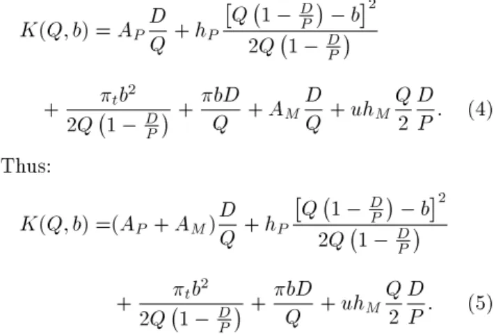
K(Q; b) = APDQ+ hP
Q 1 D P
b2 2Q 1 D
P
+ tb2
2Q 1 D P
+bDQ + AMDQ+ uhMQ2 DP: (4)
Thus:
K(Q; b) =(AP+ AM)DQ+ hP
Q 1 D P
b2 2Q 1 D
P
+ tb2
2Q 1 D P
+bDQ + uhMQ2 DP: (5)
It is required to minimize the function K(Q; b) to determine Q and b. It is easy to show that K(Q; b) is a convex function in Q and b. Therefore, it is necessary to dierentiate K(Q; b), partially, with regard to Q and b. Hence, optimizing Eq. (5), one obtains the optimal production lot size and the optimal backorders level, which are given by Eqs. (6) and (7), respectively:
Q=
s
2(AP+ AM)D(hP + t) 2D2 1 DP
hPt 1 DP+ hMuDP (hP+ t) (6);
b= (hPQ D) 1 DP
hP+ t : (7)
It is easy to see that the above expression for the production lot size immediately transforms into the well-known equation of the EPQ with shortages when
both ordering (AM) and holding (hM) costs of raw
material are zero. In other words, it is when these costs are not considered.
3.3. Comparison with EPQ with and without shortages
In this section, a numerical comparison is made be-tween the results of the proposed inventory model and those of the classical EPQ inventory model with and without shortages.
Numerical examples 1 and 2.
The data for Examples 1 and 2 are given in the rst columns of Tables 1 and 2, respectively. The results of the comparison with the EPQ without shortages are presented in Table 1. In Table 2, they are given for the comparison with the EPQ with shortages. In both tables, we use the expression of w = uCM=CP. This
means that the raw material cost is a fraction of the cost of the nished product. Typically, the holding costs are calculated as a percent of the cost (i.e., hP =
iCP yhM = iCM); then, the term w can be estimated
as w = uhM=hP.
Here, note that according to the results of Tables 1 and 2, the optimal production lot size is sensible to the fraction of cost of raw material in both inventory models. If the fraction increases, the production lot size decreases.
3.4. An EPQ inventory model with multiple raw materials and one nished product It is now appropriate to discuss that in many situations of the real life, a product is comprised of several raw materials. Although there is a unique nished product, it is made of several raw materials; therefore, one can apply the inventory models developed in the Sec-tions 3.1 and 3.2. There are always welcome practical Table 1. Comparison of the proposed inventory model with EPQ without shortages.
AP hP AM w D P Q
Q % of
dierence EPQ Proposed inventory
50 2 20 0.1 500 1000 223.61 252.26 12.82
50 2 20 0.3 500 1000 223.61 232.04 3.77
50 2 20 0.5 500 1000 223.61 216.02 3.39
50 2 20 0.7 500 1000 223.61 202.92 9.25
50 2 20 0.9 500 1000 223.61 191.94 14.1
Table 2. Comparison of the proposed inventory model with EPQ with shortages.
AP hP AM w t D P Q
b Q b Q b
EPQ Proposed inventory % of dierence 50 2 20 0.1 0.5 10 500 1000 238.48 9.45 268.72 11.98 12.68 26.74
50 2 20 0.3 0.5 10 500 1000 238.48 9.45 243.86 9.90 2.25 4.81
50 2 20 0.5 0.5 10 500 1000 238.48 9.45 224.83 8.32 5.73 11.97
50 2 20 0.7 0.5 10 500 1000 238.48 9.45 209.65 7.05 12.09 25.35
perspectives in any company for applying mathemati-cal models. Therefore, in this direction, one needs just to establish the following oversimplication, which is simple, easy to apply, and computationally ecient.
Set AM1; AM2; ; AMn as the ordering costs of
each raw material; u1; u2; ; un as the number of
units of each raw material required to manufacture one unit of the nished product; and hM1; hM2; ; hMnas
the holding cost of each raw material. Then, AM and
uhM are dened as AM = AM1+AM2+ +AMnand
uhM = u1hM1+u2hM2+ +unhMn, respectively. As
a result, one can use the previous proposed inventory models.
4. An EPQ inventory model without shortages with multi-products and raw material costs 4.1. An EPQ inventory model without
shortages with multi-products and one raw material
Here, the situation is considered in which there is a unique raw material to process several nished products and these products are manufactured in one machine or process. Consequently, it is assumed that all products share one setup cost of the production run. In this type of problem, a schedule is required for the fabrication of products. A common cycle time is used for all the products. Figure 3 illustrates the common cycle time.
It is easy to understand that in order to minimize the holding cost of raw materials, it is necessary that the product with a higher consume rate of raw material must be scheduled rst.
As an illustrative example, consider the situation of two products A and B. Suppose that one unit of product A consumes 6 units of raw material and one unit of product B requires 4 units of raw material. Moreover, the production rate of product A is 2000 units per year and the production rate of product B is 4000 units per year. Therefore, the consume rates of raw material for products A and B are 12000 units per year and 16000 units per year, respectively. As mentioned before, product B must be the rst in the production schedule (i.e., the sequence is B-A).
Then the optimization problem can be expressed as:
minK(Q1; Q2; ; Qn) = APDQj j
+
n
X
k=1
hk
2 Qk
1 DPk
k
+ AMDQj
j + hMI; (8)
subject to: D1
Q1 =
D2
Q2 = =
Dn
Qn; (9)
where I represents the required units of raw material and is given by Eq. (11). The details of the derivation of Eq. (11) are given in the Appendix.
Since:
Q2= DD2Q1 1 ; Q3=
D3Q1
D1 ; ; Qn=
DnQ1
D1 ; (10)
and: I= Q1
2D1
8 < :
n
X
k=1
D2 kuk
Pk +2 n 1X k=1
2 4Dk
Pk
0 @ Xn
j=k+1
ujDj
1 A 3 5
9 = ; :(11) Eq. (8) can be written as:
minK(Q1) = (AP + AM)DQ1 1
+2DQ1
1
( n X
k=1
hkDk
1 DPk
k
+
n
X
k=1
D2 kukhM
Pk
+ 2
n 1
X
k=1
2 4Dk
Pk
0 @ Xn
j=k+1
ujhMDj
1 A 3 5 )
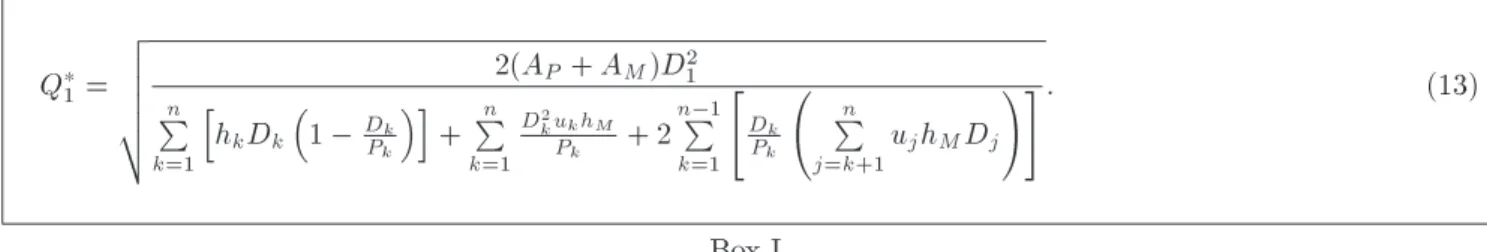
: (12) Optimizing Eq. (12), one can obtain the optimal lot size for the product 1, which is given by Eq. (13) given in Box I.
The optimal lot sizes for the rest of the products can be easily calculated by the following equation:
Q i =DDi
1Q
1: (14)
Numerical Example 3
Consider a set of products that share the same raw
Figure 3. Inventory behavior of (a) raw material, (b) nished product 1, and (3) nished product 2 considering an EPQ without shortages.
Q 1=
v u u u u t
2(AP+ AM)D21 n
P
k=1
h hkDk
1 Dk
Pk
i + Pn
k=1 D2
kukhM
Pk + 2
n 1P k=1
"
Dk
Pk
n
P
j=k+1ujhMDj
!#: (13)
Box I
Table 3. Additional information for Numerical Example 3. Units of raw
material
Total cost of
raw material uihM
Unit of production cost
Production rate
Demand rate
Product A 12 $ 120.00 $ 24.00 $ 300.00 20000 4000
Product B 6 $ 60.00 $ 12.00 $ 400.00 60000 3000
Product C 4 $ 40.00 $ 8.00 $ 200.00 30000 1500
Product D 8 $ 80.00 $ 16.00 $ 180.00 50000 2800
material and all of them must be manufactured in a unique machine. The joint setup cost of the production rate is 1000 $ per run and the ordering cost of the raw material is 400 $/order. The cost of each unit of raw material is 10 $ per unit. Assume that the annual holding cost is calculated as 20% of the cost of raw material and nished product (i.e., hk = 0:2Ck
and hM = 0:2CM). Additional information for the
numerical example is given in Table 3.
An observation is that in order to solve the inven-tory problem, it is necessary to obtain the consume rate of raw material for each product. Hence, the consume rates are 240000, 360000, 120000 and 400000 for the products A, B, C, and D, respectively. Thus, the sequence of production is D-B-A-C, and this sequence represents the order of the products in Eq. (13) as shown in Box I.
Using Eq. (13), the production lot size for prod-uct 1 is Q1= 186:96. The other lot sizes are determined
with Eq. (14) and their results are Q2= 200:32, Q3=
267:09, and Q4 = 100:16. In other words, according
to the sequence D-B-A-C, 186.96 units of product D, 200.32 units of product B, 267.09 units of product A, and 100.16 units of product C must be manufactured. 4.2. Multiple raw materials and multiple
nished products on a unique machine Now, this section deals with the case in which there exists multiple raw materials and multiple nished products, all of which are manufactures on a unique
machine. This case reduces to the previous case, there-fore, we only need to do the following:
Let AM1; AM2; ; AMn be the cost of ordering
each raw material, respectively. Let u1; u2; ; un be
the number of units of each raw material and be the holding costs of the raw materials. In this case, we dene AM as:
AM = AM1+ AM2+ + AMn;
and for each product, we establish:
uihM = u1ihM1+ u2ihM2+ + unihMn:
So, the problem is reduced to the previous case. Numerical Example 4
As an illustrative example, assume that a set of products share the same set of raw materials. In other words, there are four dierent products named as A, B, C, and D, which share three types of raw materials, called RM1, RM2, and RM3. The cost of setup of production run is 1000 $/per run and the ordering costs for raw materials RM1, RM2, and RM3 are 300 $/order, 400 $/order, and 200 $/order, respectively. Furthermore, the unit cost of each raw material is 10$/unit, 8$/unit, and 20$/unit for RM1, RM2, and RM3, respectively. Assume that the annual holding cost is determined as 15% of the costs, i.e. hk = 0:15Ck
and hMk= 0:15CMk. Additional data for the products
is shown in Table 4.
With the above information, the consume rate for Table 4. Additional information for Numerical Example 4.
Units of RM 1
Units of RM 2
Units of RM 3
Total cost of
raw materials uihM
Production cost by unit
Production rate
Demand rate
Product A 4 3 2 $ 104.00 $ 15.60 $ 400.00 20000 4000
Product B 6 1 2 $ 108.00 $ 16.20 $ 500.00 40000 3000
Product C 8 1 3 $ 148.00 $ 22.20 $ 400.00 30000 1500
production of raw material, multiplied by uihM for
each product, is calculated. The values are: 312000, 648000, 666000, and 840000 for products A, B, C, and D, respectively. Therefore, the schedule of production is D-C-B-A. Thus, AM = AM1 + AM2+ AM3 = 900.
Solving the problem, one obtains the lots sizes as Q1=
183:25, Q2 = 98:17, Q3 = 196:34, and Q4 = 261:79.
In other words, according to the sequence D-C-B-A, 183.25 units of product D, 98.17 units of product C, 196.34 units of product B, and 261.79 units of product A must be manufactured in the machine.
5. Conclusion
In the traditional EPQ model, the ordering and holding costs of the raw material are not considered. Therefore, in this paper, a generalization of the EPQ inventory model of Taft (1918) was developed. The proposed inventory model considers both costs of raw material: ordering and holding. A main conclusion is that these costs must be taken into account, because they impact, directly, on the optimal production lot size. In both inventory models, EPQ without shortages and EPQ with shortages were observed. It is concluded that the production lot size is very sensible to the costs of raw material. The main new contribution of this paper is presenting an EPQ inventory model that determines the optimal lot size for a product that requires more than one raw material and an EPQ inventory model that determines the lot size for multiple products and multiple raw materials.
Acknowledgments
The research for the second author was supported by Tecnologico de Monterrey Research Group in Industrial Engineering and Numerical Methods 0822B01006. The authors would like to thank the three anonymous referees for their valuable and helpful suggestions. These suggestions have strongly improved this paper. References
1. Harris, F.W. \How many parts to make at once", Factory, The Magazine of Management, 10(2), pp. 135-136, 152 (1913).
2. Taft, E.W. \The most economical production lot", Iron Age, 101, pp. 1410-1412 (1918).
3. Wilson, R.H. \A scientic routine for stock control", Harvard Business Review, 13, pp. 116-128 (1934).
4. Cardenas-Barron, L.E., Chung, K.J. and Trevi~no-Garza, G. \Celebrating a century of the economic order quantity model in honor of Ford Whitman Harris", International Journal of Production Economics, 155, pp. 1-7 (2014).
5. Banerjee, A., Sylla, C. and Eiamkanchanalai, S. \In-put/output lot sizing in single stage batch production systems under constant demand", Computers and Industrial Engineering, 19(1-4), pp. 37-41 (1990).
6. Golhar, D.Y. and Sarker, B.R. \Economic manufac-turing quantity in a just-in-time delivery system", International Journal of Production Research, 30(5), pp. 961-972 (1992).
7. Jamal, A.M.M. and Sarker, B.R. \An optimal batch size for a production system operating under a just-in-time delivery system", International Journal of Production Economics, 32(2), pp. 255-260 (1993).
8. Sarker, B.R. and Golhar, D.Y. \A reply to a note to \Economic manufacturing quantity in a just-in-time delivery system"", International Journal of Production Research, 31(11), p. 2749 (1993).
9. Sarker, B.R. and Parija, G.R. \An optimal batch size for a production system operating under a xed-quantity, periodic delivery policy", Journal of Opera-tional Research Society, 45(8), pp. 891-900 (1994).
10. Sarker, R.A., Karim, A.N.M. and Haque, A.F.M.A. \An optimal batch size for a production system operat-ing under a continuous supply/demand", International Journal of Industrial Engineering, 2(3), pp. 189-198 (1995).
11. Sarker, B.R. and Parija, G.R. \Optimal batch size and raw material ordering policy for a production system with a xed-interval, lumpy demand delivery system", European Journal of Operational Research, 89(3), pp. 593-608 (1996).
12. Sarker, R.A. and Khan, L.R. \An optimal batch size for a production system operating under periodic de-livery policy", Computers and Industrial Engineering, 37(4), pp. 711-730 (1999).
13. Khan, L.R., Sarker, R.A. \An optimal batch size for a JIT manufacturing system", Computers and Industrial Engineering, 42(2-4), pp. 127-136 (2002).
14. Eilon, S. \Scheduling for batch production", Journal of Institute of Production Engineering, 36, pp. 549-570, 582 (1957).
15. Rogers, J. \A computational approach to the economic lot scheduling problem", Management Science, 4(3), pp. 264-291 (1958).
16. Bomberger, E.E. \A dynamic programming approach to a lot size scheduling problem", Management Sci-ence, 12(11), pp. 778-784 (1966).
17. Madigan, J.G. \Schedulling a multi-product single machine system for an innite planning period", Man-agement Science, 14(11), pp. 713-719 (1968).
18. Stankard, M.F. and Gupta, S.K. \A note on Bomberger's approach to lot size scheduling: Heuristic proposed", Management Science, 15(7), pp. 449-452 (1969).
19. Hodgson, T.J. \Addendum to standard and Gupta's note on lot size scheduling", Management Science, 16(7), pp. 514-517 (1970).
20. Baker, K.R. \On Madigan's approach to the de-terministic multi-product production and inventory problem", Management Science, 16(9), pp. 636-638 (1970).
21. Davis, S.G. \Scheduling economic lot size produc-tion runs", Management Science, 36(8), pp. 985-998 (1990).
22. Fransoo, J.C., Sridharan, V. and Bertrand, J.W.M. \A hierarchical approach for capacity coordination in mul-tiple products single-machine production systems with stationary stochastic demands", European Journal of Operational Research, 86(1), pp. 57-72 (1995).
23. Sarker, R.A. and Newton, C. \A genetic algorithm for solving economic lot size scheduling problem", Computers and Industrial Engineering, 42(2-4), pp. 189-198 (2002).
24. Cooke, D.L., Rohleder, T.R. and Silver, E.A. \Find-ing eective schedules for the economic lot schedul-ing problem: A simple mixed integer programmschedul-ing approach", International Journal of Production Re-search, 42(1), pp. 21-36 (2004).
25. Hishamuddin, H., Sarker, R.A. and Essam, D. \A dis-ruption recovery model for a single stage production-inventory system", European Journal of Operational Research, 222(3), pp. 464-473 (2012).
26. Taleizadeh, A.A., Wee, H.M. and Sadjadi, S.J. \Multi-product \Multi-production quantity model with repair failure and partial backordering", Computers and Industrial Engineering, 59(1), pp. 45-54 (2010a).
27. Taleizadeh, A.A., Naja, A.A. and Niaki, S.T.A. \Eco-nomic production quantity model with scrapped items and limited production capacity", Scientia Iranica E, 17(1), pp. 58-69 (2010).
28. Taleizadeh, A.A., Niaki, S.T.A. and Naja, A.A. \Multiproduct single-machine production system with stochastic scrapped production rate, partial backorder-ing and service level constraint", Journal of Compu-tational and Applied Mathematics, 233(8), pp. 1834-1849 (2010).
29. Chiu, S.W., Lin, H.-D., Wu, M.-F. and Yang, J.-Ch. \Determining replenishment lot size and shipment policy for an extended EPQ model with delivery and quality assurance issues", Scientia Iranica E, 18(6), pp. 1537-1544 (2011).
30. Taleizadeh, A.A., Sadjadi, S.J. and Niaki, S.T.A. \Multiproduct EPQ model with single machine, back-ordering and immediate rework process", European Journal of Industrial Engineering, 5(4), pp. 388-411 (2011a).
31. Taleizadeh, A.A., Shavandi, H. and Haji, R. \Con-strained single period problem under demand un-certainty", Scientia Iranica E, 18(6), pp. 1553-1563 (2011b).
32. Sepehri, M. \Cost and inventory benets of coop-eration in multi-period and multi-product supply", Scientia Iranica E, 18(3), pp. 731-741 (2011).
33. Taleizadeh, A.A., Cardenas-Barron, L.E., Biabani, J. and Nikousokhan, R. \Multi products single machine EPQ model with immediate rework process", Inter-national Journal of Industrial Engineering Computa-tions, 3(2), pp. 93-102 (2012).
34. Ramezanian, R. and Saidi-Mehrabad, M. \Multi-product unrelated parallel machines scheduling prob-lem with rework processes", Scientia Iranica E, 19(6), pp. 1887-1893 (2012).
35. Taleizadeh, A.A., Wee, H.M. and Jalali-Naini, S.G. \Economic production quantity model with repair failure and limited capacity", Applied Mathematical Modelling, 37(5), pp. 2765-2774 (2013).
36. Taleizadeh, A.A., Jalali-Naini, S.G., Wee, H.M. and Kuo, T.C. \An imperfect multi-product production system with rework", Scientia Iranica E, 20(3), pp. 811-823 (2013).
37. Taleizadeh, A.A., Cardenas-Barron, L.E. and Mo-hammadi, B. \A deterministic multi product single machine EPQ model with backordering, scraped prod-ucts, rework and interruption in manufacturing pro-cess", International Journal of Production Economics, 150(1), pp. 9-27 (2014).
38. Holmbom, M., Segerstedt, A. and Sluis, E. \A solution procedure for economic lot scheduling problems even in high utilization facilities", International Journal of Production Research, 51(12), pp. 3765-3777 (2013).
39. Holmbom, M. and Segerstedt, A. \Economic order quantities in production: From Harris to economic lot scheduling problems", International Journal of Production Economics, 155, pp. 82-90 (2014).
40. Pal, B., Sana, S.S. and Chaudhuri, K. \A stochastic in-ventory model with product recovery", CIRP Journal of Manufacturing Science and Technology, 6(2), pp. 120-127 (2013).
41. Roy, M.D., Sana, S.S. and Chaudhuri, K. \An eco-nomic production lot size model for defective items with stochastic demand, backlogging and rework", IMA Journal of Management Mathematics, 25(2), pp. 159-183 (2014).
42. Hsu, L.F. \A note on \An Economic Order Quantity (EOQ) for items with imperfect quality and inspection errors"", International Journal of Industrial Engineer-ing Computations, 3(4), pp. 695-702 (2012).
43. Hsu, J.T. and Hsu, L.F. \An integrated single-vendor single-buyer production-inventory model for items with imperfect quality and inspection errors", International Journal of Industrial Engineering Com-putations, 3(5), pp. 703-720 (2012).
44. Sana, S.S. \A collaborating inventory model in a supply chain", Economic Modelling, 29(5), pp. 2016-2023 (2012).
45. Kumar, N., Singh, S.R. and Kumari, R. \Two-warehouse inventory model of deteriorating items with three-component demand rate and time-proportional backlogging rate in fuzzy environment", International Journal of Industrial Engineering Computations, 4(4), pp. 587-598 (2013).
46. Tripathi, R.P. \Inventory model with dierent demand rate and dierent holding cost", International Journal of Industrial Engineering Computations, 4(3), pp. 437-446 (2013).
47. Sana, S.S. \Optimal production lot size and reorder point of a two-stage supply chain while random de-mand is sensitive with sales teams' initiatives", Inter-national Journal of Systems Science, 47(2), pp. 450-465 (2016).
48. Sana, S.S., Chedid, J.A. and Salas Navarro, K. \A three layer supply chain model with multiple suppli-ers, manufacturers and retailers for multiple items", Applied Mathematics and Computation, 229, pp. 139-150 (2014).
49. Farughi, H., Khanlarzade, N. and Yegane, B.Y. \Pric-ing and inventory control policy for non-instantaneous deteriorating items with time- and price-dependent demand and partial backlogging", Decision Science Letters, 3(3), pp. 325-334 (2014).
Appendix A
Detailed derivation of inventory average ( I) The inventory level of raw material at any time t, as depicted in Figure A.1., is partitioned into the quantities manufactured by time for each of the three nished products and the total inventory is consumed in that time.
Thus, the inventory average is determined as follows:
Q1=P1
Q1=D1
[(u1Q1+ u2Q2+ u3Q3) + (u2Q2+ u3Q3)]
2 +QQ2=P2
1=D1
[(u2Q2+ u3Q3) + (u3Q3)]
2 +QQ3=P3
1=D1
[u3Q3]
2 =
D1
P1
u1Q1+ 2u2Q2+ 2u3Q3
2 +DP1Q2
2Q1
u2Q2+ 2u3Q3
2 +
D1Q3
P3Q1
u3Q3
2 :
Figure A.1. Inventory pattern of raw material with three nished products.
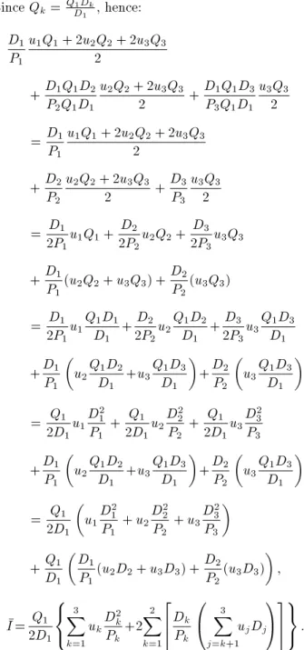
Since Qk= QD1D1k, hence:
D1
P1
u1Q1+ 2u2Q2+ 2u3Q3
2 +DP1Q1D2
2Q1D1
u2Q2+ 2u3Q3
2 +
D1Q1D3
P3Q1D1
u3Q3
2 =DP1
1
u1Q1+ 2u2Q2+ 2u3Q3
2 +DP2
2
u2Q2+ 2u3Q3
2 +
D3
P3
u3Q3
2 = D1
2P1u1Q1+
D2
2P2u2Q2+
D3
2P3u3Q3
+DP1
1(u2Q2+ u3Q3) +
D2
P2(u3Q3)
=2PD1
1u1
Q1D1
D1 +
D2
2P2u2
Q1D2
D1 +
D3
2P3u3
Q1D3
D1
+DP1
1
u2QD1D2 1 +u3
Q1D3
D1
+DP2
2
u3QD1D3 1
= Q1 2D1u1
D2 1
P1 +
Q1
2D1u2
D2 2
P2 +
Q1
2D1u3
D2 3
P3
+DP1
1
u2QD1D2 1 +u3
Q1D3
D1
+DP2
2
u3QD1D3 1
=2DQ1
1
u1D
2 1
P1 + u2
D2 2
P2 + u3
D2 3
P3
+DQ1
1
D1
P1(u2D2+ u3D3) +
D2
P2(u3D3)
; I= Q1
2D1 8 < : 3 X k=1
ukD 2 k
Pk+2 2 X k=1 2 4Dk Pk 0 @ X3
j=k+1
ujDj
1 A 3 5 9 = ;: For induction, the inventory average for n products is calculated as shown in Box II. After some algebraic manipulations, one obtains:
D1
P1
u1Q1
2 + u2Q2+ u3Q3+ + unQn
+QP2D1
2Q1
u2Q2
2 + u3Q3+ + unQn
+Q3D1 P3Q1
u3Q3
2 + u4Q4+ + unQn
+ +QPn 1D1
n 1Q1
un 1Qn 1
2 + unQn
Q1=P1
Q1=D1
[(u1Q1+ u2Q2+ u3Q3+ + unQn) + (u2Q2+ u3Q3+ + unQn)]
2 +QQ2=P2
1=D1
[(u2Q2+ u3Q3+ + unQn) + (u3Q3+ + unQn)]
2 +QQ3=P3
1=D1
[(u3Q3+ + unQn) + (u4Q4+ + unQn)]
2 +
+Qn 1Q =Pn 1
1=D1
[un 1Qn 1+ unQn+ unQn]
2 +
Qn=Pn
Q1=D1
unQn
2 : Box II
+QPnD1
nQ1
unQn
2
: Since that D1
Q1 =
D2
Q2 = =
Dn
Qn, thus Qk =
DkQ1
D1 .
Therefore, by substituting Qk, we have:
D1
P1
u1Q1
2 + u2Q2+ u3Q3+ + unQn
+D2Q1D1 P2Q1D1
u2Q2
2 + u3Q3+ + unQn
+DP3Q1D1
3Q1D1
u3Q3
2 + u4Q4+ + unQn
+DPn 1Q1D1
n 1Q1D1
un 1Qn 1
2 + unQn
+DPnQ1D1
nQ1D1
unQn
2 : Simplifying: D1 P1 u1Q1
2 + u2Q2+ u3Q3+ + unQn
+DP2
2
u2Q2
2 + u3Q3+ + unQn
+DP3
3
u3Q3
2 + u4Q4+ + unQn
+DPn 1
n 1
un 1Qn 1
2 + unQn
+DPn
n
unQn
2
; after some algebraic manipulations:
D1
P1
u1Q1
2 + D2
P2
u2Q2
2 + D3
P3
u3Q3
2 + + Dn
Pn
unQn
2
+DP1
1[u2Q2+ u3Q3+ + unQn]
+D2
P2[u3Q3+ + unQn] +
+DPn 1
n 1[unQn];
the rst part can be expressed as: D1
P1
u1Q1
2 + D2
P2
u2Q2
2 + D3
P3
u3Q3
2 + +DPn
n
unQn
2 =
n
X
k=1
DkukQk
2Pk :
Substituting the expression of Qk: n
X
k=1
DkukQk
2Pk = n
X
k=1
D2 kukQ1
2D1Pk =
Q1 2D1 n X k=1 D2 kuk
Pk ;
the second part can be expressed as: D1
P1[u2Q2+ u3Q3+ + unQn]
+DP2
2[u3Q3+ + unQn] +
+Dn 1 Pn 1[unQn]
= n 1 X k=1 2 4Dk Pk 0 @ Xn
j=k+1
ujQj
1 A 3 5
=n 1X
k=1
2 4Dk
Pk
0 @ Xn
j=k+1
ujQD1Dj 1
1 A 3 5
=DQ1
1 n 1 X k=1 2 4Dk Pk 0 @ Xn
j=k+1
ujDj
1 A 3 5
= 22DQ1
1 n 1X k=1
2 4Dk
Pk
0 @ Xn
j=k+1
ujDj
1 A 3 5 : Thus, the inventory average is given by:
I = Q1
2D1
( n X
k=1
D2 kuk
Pk
+2n 1X
k=1
2 4Dk
Pk
0 @ Xn
j=k+1
ujDj
1 A 3 5
9 = ; : Biographies
Ernesto Armando Pacheco-Velazquez is currently a Professor in the Department of Industrial and Sys-tems Engineering at Tecnologico de Monterrey, Cam-pus Ciudad de Mexico, Mexico. He has been teaching and researching at Tecnologico de Monterrey for more
than 25 years. He has published several papers. His research areas primarily include inventory, logistics, supply chain, decision making, and voting.
Leopoldo Eduardo Cardenas-Barron is currently a Professor at the School of Engineering and Sciences at Tecnologico de Monterrey, Campus Monterrey, Mexico. He is also a faculty member in the Department of Industrial and Systems Engineering at Tecnologico de Monterrey. He was the associate director of the Indus-trial and Systems Engineering programme from 1999 to 2005. Moreover, he was the associate director of the Department of Industrial and Systems Engineering from 2005 to 2009. His research areas primarily include inventory planning and control, logistics, and supply chain. He has published papers and technical notes in several national and international journals. He has co-authored one book in the eld of Simulation in Spanish. He is also editorial board member in several international journals.