Unit 27: Comparing
Two Means
Prerequisites
Students should have experience with one-sample t-procedures before they begin this unit. That material is covered in Unit 26, Small Sample Inference for One Mean.
Additional Topic Coverage
Additional coverage of two-sample t-procedures can be found in The Basic Practice of
Statistics, Chapter 19, Two-Sample Problems.
Activity Description
In this activity, students will check whether the mean number of chips per cookie in Nabisco’s Chips Ahoy regular and reduced fat chocolate chip cookies differ. In Unit 25’s activity, students collected data on the number of chips per cookie from Chips Ahoy regular chocolate chip cookies. They can use those data in this activity. In addition, if they have not already done so, they will need to collect data on the number of chips per cookie from one or more bags of Chips Ahoy reduced fat chocolate chip cookies.
Materials
One or two bags each of Nabisco’s Chips Ahoy chocolate chip cookies, regular and reduced fat; paper plates or paper towels.
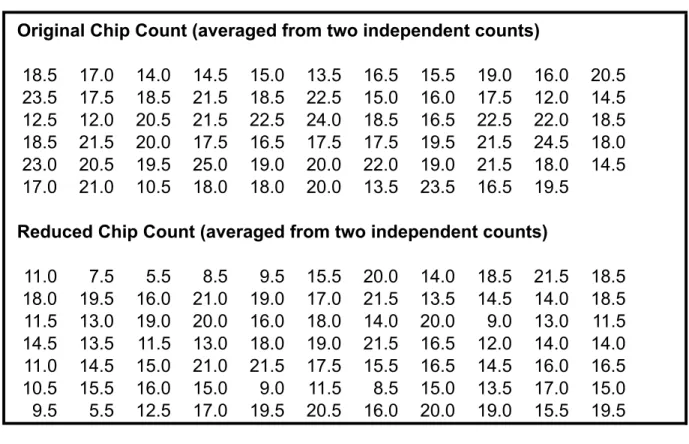
If students have not collected the data as part of Unit 25’s activity, then they should be assigned to work in groups of 2 to 4 students to collect the data for this activity. If you need to have a group of 3, students in the group can trade off being chip counters. See Unit 25’s Activity Description for suggestions on collecting these data. The sample data, on which sample solutions to the activity are based, are given in Table T27.1. For the sample data, two
independent counts were taken on the number of chips in each cookie, and then the results were averaged.
Table T27.1. Sample data.
Students will need a copy of the class data for questions 2 – 5. If you decide not to collect the data (a task students really enjoy), have the class use the sample data in Table T27.1, which was collected in two statistics classes (each class got a bag of each type of cookie).
18.5 17.0 14.0 14.5 15.0 13.5 16.5 15.5 19.0 16.0 20.5 23.5 17.5 18.5 21.5 18.5 22.5 15.0 16.0 17.5 12.0 14.5 12.5 12.0 20.5 21.5 22.5 24.0 18.5 16.5 22.5 22.0 18.5 18.5 21.5 20.0 17.5 16.5 17.5 17.5 19.5 21.5 24.5 18.0 23.0 20.5 19.5 25.0 19.0 20.0 22.0 19.0 21.5 18.0 14.5 17.0 21.0 10.5 18.0 18.0 20.0 13.5 23.5 16.5 19.5
11.0 7.5 5.5 8.5 9.5 15.5 20.0 14.0 18.5 21.5 18.5 18.0 19.5 16.0 21.0 19.0 17.0 21.5 13.5 14.5 14.0 18.5 11.5 13.0 19.0 20.0 16.0 18.0 14.0 20.0 9.0 13.0 11.5 14.5 13.5 11.5 13.0 18.0 19.0 21.5 16.5 12.0 14.0 14.0 11.0 14.5 15.0 21.0 21.5 17.5 15.5 16.5 14.5 16.0 16.5 10.5 15.5 16.0 15.0 9.0 11.5 8.5 15.0 13.5 17.0 15.0 9.5 5.5 12.5 17.0 19.5 20.5 16.0 20.0 19.0 15.5 19.5 Table T27.1
Reduced Chip Count (averaged from two independent counts) Original Chip Count (averaged from two independent counts)
The Video Solutions
1. Sample answer: Take a sample from all licensed drivers in some state and look at the
number of tickets the males and females in this group received for moving violations. We could then compare the mean number of tickets for women to the mean number of tickets for men.
2. The Hadza are a group of traditional hunter-gatherers who live in a way that is very similar to our ancestors. The men hunt with bows and arrows and the women forage for berries and root vegetables.
3. The original assumption was that the Hadza would burn more calories than the Westerners do, due to their more active lifestyle.
4. A two-sample t-test was used.
5. It turned out that no significant difference was found between the mean daily total energy expenditures of the Hadza and the Westerners. So, the researchers’ original assumption that the Hadza burned more calories than Westerners due to a more active lifestyle was not supported by the data.
Unit Activity Solutions
1. See question 3.
2. a. Sample answer: Since chocolate chips have fat in them, we think that Nabisco may put fewer chips in its reduced fat cookies as a way of reducing the fat content.
b. Sample answer: Given our answer in (a), we decided to use a one-sided alternative. Let
µ1 = the mean number of chips per cookie in regular Chips Ahoy chocolate chip cookies
and let µ2 = the mean number of chips per cookie in reduced fat Chips Ahoy chocolate chip cookies. Below are the null and alternative hypotheses:
H0:µ1−µ2 =0
Ha:µ1−µ2 >0
3. Sample data:
Original Chip Count (averaged from two independent counts)
18.5 17.0 14.0 14.5 15.0 13.5 16.5 15.5 19.0 16.0 20.5 23.5 17.5 18.5 21.5 18.5 22.5 15.0 16.0 17.5 12.0 14.5 12.5 12.0 20.5 21.5 22.5 24.0 18.5 16.5 22.5 22.0 18.5 18.5 21.5 20.0 17.5 16.5 17.5 17.5 19.5 21.5 24.5 18.0 23.0 20.5 19.5 25.0 19.0 20.0 22.0 19.0 21.5 18.0 14.5 17.0 21.0 10.5 18.0 18.0 20.0 13.5 23.5 16.5 19.5
Reduced Chip Count (averaged from two independent counts)
11.0 7.5 5.5 8.5 9.5 15.5 20.0 14.0 18.5 21.5 18.5 18.0 19.5 16.0 21.0 19.0 17.0 21.5 13.5 14.5 14.0 18.5 11.5 13.0 19.0 20.0 16.0 18.0 14.0 20.0 9.0 13.0 11.5 14.5 13.5 11.5 13.0 18.0 19.0 21.5 16.5 12.0 14.0 14.0 11.0 14.5 15.0 21.0 21.5 17.5 15.5 16.5 14.5 16.0 16.5 10.5 15.5 16.0 15.0 9.0 11.5 8.5 15.0 13.5 17.0 15.0 9.5 5.5 12.5 17.0 19.5 20.5 16.0 20.0 19.0 15.5 19.5
Regular: n1=65, x1=18.462, s1=3.308
Reduced Fat: n2 =77, x2 =15.266, s2 =3.941
4. Based on comparative boxplots, it appears that Chips Ahoy regular has more chips per cookie than Chips Ahoy reduced fat.
Reduced Fat Original
25 20
15 10
5
Co
ok
ie
Ty
pe
Number of Chips
5. a. Sample answer:
t =(18.462−15.266)−0
3.3082
65 +3.941 2 77
≈5.25
b. Sample answer: Using a conservative approach, we assume that df = 65 – 1 = 64. From software and using a one-sided alternative, we get a p-value that is essentially 0 (at least to 4 decimals).
c. Sample answer: Reject the null hypothesis. Conclude that the difference in the mean number of chips per cookie between the two types of cookies is positive. Hence, the mean number of chips per cookie in Chips Ahoy regular cookies is greater than the mean number of chips per cookie in Chips Ahoy reduced fat cookies.
6. Sample answer: (18.462−15.266)±(1.998) (3.308)2 65 +
(3.941)2
77 ≈3.196±1.215, or
Exercise Solutions
1. a. Let µ1 be the mean job performance rating for pregnant employees and µ2 be the mean job performance rating for non-pregnant female employees.
H0:µ1−µ2 =0
Ha:µ1−µ2 ≠0
b. t =(2.38−2.69)−0
1.102
71 +0.58 2 71
≈ −2.10
Using a two-sided alternative, and letting df = 71-1 = 70 (the conservative approach), we determine p = 2(0.01967) ≈ 0.039. (If we use the statistical package Minitab, we get df = 106 and p = 0.038. The conservative approach yields a slightly higher p-value.) We conclude that there is a statistical difference in the mean job performance ratings for the two groups.
c. Using the conservative approach, we set df = 70 in order to determine the t-critical value:
t* ≈ 1.994.
2 2
1.10 0.58
(2.38 2.69) (1.994) 0.31 0.294
71 71
− ± + ≈ − ± , or (-0.604, -0.016)
Since both endpoints of the confidence interval are negative, the mean job performance appraisal rating for pregnant employees is lower than for non-pregnant female employees. In this case, lower ratings are associated with better job performance.
2. a. A one-sample paired t-test should be used. The “during” and “after” data involve the same group of women rather than samples from two independent populations.
b. t = −0.27−0
2.00 71
≈ −1.138 ;
based on a t-distribution with df = 70 and a two-sided alternative, p = 2(0.1295) ≈ 0.259. The mean difference in job performance appraisal ratings during pregnancy and after returning
3. a. Sample answer: It is somewhat difficult to tell if the distribution of SAT Math scores is higher for males than for females. From the dotplots, the distribution of SAT Math scores is more variable for males than for females. The highest SAT Math scores are from males but the lowest are also from males. Nevertheless, the midpoint of the distribution for the male students appears higher than the midpoint of the distribution for the female students.
b. Consider the normal quantile plots below. Given the dots fall within 95% confidence interval bands on the normal quantile plots, it is reasonable to assume the data from both samples come from approximately normal distributions.
c. xF =493.5, sF =44.64; xM =544.0, sM =80.6
d. (544.0 493.5) 0 2.452 2
80.6 44.64
20 20
t = − − ≈
+
; using df = 19, we get the following p-value: p ≈ 0.012
Therefore, we can conclude that the mean SAT Math scores are significantly higher for first-year male students entering this university than for first-first-year female students.
680 640 600 560 520 480 440 400 Female Male Math SAT Ge nd er 600 500 400 99 95 90 80 70 60 50 40 30 20 10 5 1 800 600 400 99 95 90 80 70 60 50 40 30 20 10 5 1
Math SAT Females
Pe
rc
en
t
Math SAT Males
Normal - 95% CI
4. a. H0:µG −µB =0 versus Ha:µG −µB ≠0. (Could also be expressed as H0:µG =µB versus
Ha:µG ≠µB.) b.
2 2
(494 409) 0 2.023 (172) (148)
31 27
t = − − ≈
+
c. Use df = 27 – 1, or 26; p = 2(0.02673) ≈ 0.053. Since p > 0.5, the results are not significant at the 0.05 level.
d.
+
= ≈
+
2
2 2
2 2
2 2
172 148
31 27
55.9948
1 172 1 148
30 31 26 27
df ; use df = 55.
p = 2(0.02397) ≈ 0.048. Since p < 0.05, the results are significant at the 0.05 level.
Notice that the p-value in (c) is only slightly larger using the conservative approach than it is here.
Review Questions Solutions
1. The men in the sample earned more, on average, than did the women. The difference in the sample means was large enough that it couldn’t be attributed to chance variation. If we assume that men and women in the entire student population have the same average earnings, the probability of observing a difference as large as we observed is only p = 0.038, making it pretty unlikely (less than a 4% chance). Because this probability is so small, we have good evidence that the average earnings of all male and female students (not just those who happen to be in the samples) differ.
There was also some difference between the average earnings of African- American and white students in the sample. However, a difference at least this large would happen almost half the time (p = 0.476) just by chance if African Americans and whites in the entire student population had exactly the same average earnings.
2. a. Sample answer: No mention was made that the samples were randomly selected from each area. The researchers wanted to be sure that the differences in pulmonary function could be attributed to the pollution levels in the two areas and not due to a lurking variable such as age, height, weight or BMI that was different for the men in the two groups of participants in the study.
b. (4.49 4.32) 0 2.1162 2
0.43 0.45
60 60
t = − − ≈
+
; using df = 59, we get p = 2(0.01929) ≈ 0.039
We conclude that there is a statistically significant difference in mean forced vital capacity (FVC) in healthy, non-smoking, young men in Area 1 and Area 2. (Because the sample size was large, even a relatively small difference in sample means turned out to be statistically different.)
c.
2 2
(17.17 16.28) 0 1.411 4.26 2.39
60 60
t = − − ≈
+
; using df = 59, we get p = 2(0.08175) ≈ 0.164
We conclude that there is no significant difference in the mean respiratory rate in healthy, non-smoking, young men in Areas 1 and 2.
d. We construct a 95% confidence interval for the difference in mean FVC between the two areas. We use df = 59 (conservative approach) to find the t-critical value: t* = 2.001.
− ± 0.432 +0.452 ≈ ±
(4.49 4.32) (2.001) 0.17 0.16
60 60 or (0.01, 0.33).
3. a. Both distributions appear reasonably symmetric. Neither data set has outliers. The whiskers on the boxplots appear slightly longer than half the width of the boxes. These are characteristics that you would expect from normal data. So, based on the boxplots it appears reasonable to assume that both data sets are approximately normal. Although the SAT Writing scores for the male students are more spread out than for the female students, it looks as if the SAT Writing scores for the female students tend to be higher than for the male students.
b. Female students: nF =25, xF =541.20, sF =48.59
Male students: nM =35, xF =507.10, sM =73.70
c.
2 2
(541.20 507.1) 0 2.16 (48.59) (73.7)
25 35
t = − − ≈
+
Adopting a conservative approach, we use df = 24 to determine a p-value: We get
p = 2(0.02049) ≈ 0.041 < 0.05. We conclude that there is a significant difference between the mean SAT Writing scores for first-year women at this university compared to first-year men. d. (541.20 507.10) 2.064− ± 48.592 +73.72 ≈34.10 32.61±
25 35 , or (1.49, 66.71) Male
Female
650 600
550 500
450 400
350
Ge
nde
r
4. a. H0:µB−µG =0 versus Ha:µB−µG >0.
(Could also be expressed as H0:µB =µG versus H0:µB =µG.)
b. = − − ≈ +
2 2
(92.3 80.8) 0 1.05 42.0 41.4
27 31
t ; using df = 26, p = 0.152
There is insufficient evidence to reject the null hypothesis in favor of the alternative. Hence, we are unable to conclude from these data that 4-year-old boys consume more mouthfuls of food during a meal than 4-year-old girls.