Natural Language Processing (almost) from Scratch
Ronan Collobert [email protected]
NEC Labs America, Princeton NJ.
Jason Weston [email protected]
Google, New York, NY.
L´eon Bottou [email protected]
Michael Karlen [email protected]
Koray Kavukcuoglu† [email protected]
Pavel Kuksa‡ [email protected]
NEC Labs America, Princeton NJ.
Editor:
Abstract
We propose a unified neural network architecture and learning algorithm that can be applied to various natural language processing tasks including: part-of-speech tagging, chunking, named entity recognition, and semantic role labeling, achieving or exceeding state-of-the-art performance in each on four benchmark tasks. Our goal was to design a flexible architecture that canlearnrepresentations useful for the tasks, thus avoiding excessive task-specific feature engineering (and therefore disregarding a lot of prior knowledge). Instead of exploiting man-made input features carefully optimized for each task, our system learns internal representations on the basis of vast amounts of mostly unlabelled training data. This work is then used as a basis for building a freely available tagging system with excellent performance while requiring minimal computational resources.
Keywords: Natural Language Processing, Neural Networks, Deep Learning
1. Introduction
Who nowadays still hopes to design a computer program able to convert a piece of English text into a computer-friendly data structure that unambiguously and completely describes the meaning of the text? Among numerous problems, no consensus has emerged about the form of such a data structure. Until such fundamental problems are resolved, computer scientists must settle for reduced objectives: extracting simpler representations describing restricted aspects of the textual information.
These simpler representations are often motivated by specific applications, for instance, bag-of-words variants for information retrieval. These representations can also be motivated by our belief that they capture something more general about the natural language. They can describe syntactical information (e.g. part-of-speech tagging, chunking, and parsing) or semantic information (e.g. word-sense disambiguation, semantic role labeling, named entity
†. Koray Kavukcuoglu is also with New York University, New York, NY. ‡. Pavel Kuksa is also with Rutgers University, New Brunswick, NJ.
extraction, and anaphora resolution). Text corpora have been manually annotated with such data structures in order to compare the performance of various systems. The availability of standard benchmarks has stimulated research in Natural Language Processing (NLP).
Many researchers interpret such reduced objectives as stepping stones towards the goal of understanding natural languages. Real-world NLP applications have been approached by smartly reconfiguring these systems and combining their outputs. The benchmark results then tell only a part of the story because they do not measure how effectively these systems can be reconfigured to address real world tasks.
In this paper, we try to excel in multiple benchmark tasks using asingle learning system. In fact we view the benchmarks as indirect measurements of the relevance of the internal representations discovered by the learning procedure, and we posit that these intermediate representations are more general than any of the benchmark targets.
Many highly engineered NLP systems address the benchmark tasks using linear statistical models applied to task-specific features. In other words, the researchers themselves discover intermediate representations by engineering ad-hoc features. These features are often derived from the output of preexisting systems, leading to complex runtime dependencies. This approach is effective because researchers leverage a large body of linguistic knowledge. On the other hand, there is a great temptation to over-engineer the system to optimize its performance on a particular benchmark at the expense of the broader NLP goals.
In this contribution, we describe a unified NLP system that achieves excellent performance on multiple benchmark tasks by discovering its own internal representations. We have avoided engineering features as much as possible and we have therefore ignored a large body of linguistic knowledge. Instead we reach state-of-the-art performance levels by transfering intermediate representations discovered on massive unlabeled datasets. We call this approach “almost from scratch” to emphasize this reduced (but still important) reliance on a priori NLP knowledge.
The paper is organized as follows. Section 2 describes the benchmark tasks of interest. Section 3 describes the unified model and reports benchmark results obtained with supervised training. Section 4 leverages very large unlabeled datasets to train the model on a language modeling task. Vast performance improvements are demonstrated by transfering the unsupervised internal representations into the supervised benchmark models. Section 5 investigates multitask supervised training. Section 6 evaluates how much further improvement could be achieved by incorporating classical NLP engineering tricks into our systems. We then conclude with a short discussion section.
2. The Benchmark Tasks
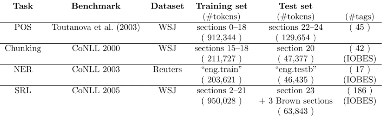
In this section, we briefly introduce four classical NLP tasks on which we will benchmark our architectures within this paper: Part-Of-Speech tagging (POS), chunking (CHUNK), Named Entity Recognition (NER) and Semantic Role Labeling (SRL). For each of them, we consider a classical experimental setup and give an overview of state-of-the-art systems on this setup. The experimental setups are summarized in Table 1, while state-of-the-art systems are reported in in Table 2.
Task Benchmark Dataset Training set Test set
(#tokens) (#tokens) (#tags)
POS Toutanova et al. (2003) WSJ sections 0–18 sections 22–24 ( 45 ) ( 912,344 ) ( 129,654 )
Chunking CoNLL 2000 WSJ sections 15–18 section 20 ( 42 )
( 211,727 ) ( 47,377 ) (IOBES)
NER CoNLL 2003 Reuters “eng.train” “eng.testb” ( 17 )
( 203,621 ) ( 46,435 ) (IOBES)
SRL CoNLL 2005 WSJ sections 2–21 section 23 ( 186 )
( 950,028 ) + 3 Brown sections (IOBES) ( 63,843 )
Table 1: Experimental setup: for each task, we report the standard benchmark we used, the dataset it relates to, as well as training and test information.
System Accuracy
Shen et al. (2007) 97.33%
Toutanova et al. (2003) 97.24%
Gim´enez and M`arquez (2004) 97.16%
(a) POS
System F1
Shen and Sarkar (2005) 95.23%
Sha and Pereira (2003) 94.29%
Kudo and Matsumoto (2001) 93.91%
(b) CHUNK
System F1
Ando and Zhang (2005) 89.31%
Florian et al. (2003) 88.76%
Kudo and Matsumoto (2001) 88.31%
(c) NER
System F1
Koomen et al. (2005) 77.92%
Pradhan et al. (2005) 77.30% Haghighi et al. (2005) 77.04%
(d) SRL
Table 2: State-of-the-art systems on four NLP tasks. Performance is reported in per-word accuracy for POS, and F1 score for CHUNK, NER and SRL. Systems in bold will be referred asbenchmark systems in the rest of the paper (see text).
2.1 Part-Of-Speech Tagging
POS aims at labeling each word with a unique tag that indicates its syntactic role, e.g. plural noun, adverb, . . . A classical benchmark setup is described in detail by Toutanova
et al. (2003). Sections 0–18 of WSJ data are used for training, while sections 19–21 are for validation and sections 22–24 for testing.
The best POS classifiers are based on classifiers trained on windows of text, which are then fed to a bidirectional decoding algorithm during inference. Features include preceding and following tag context as well as multiple words (bigrams, trigrams. . . ) context, and handcrafted features to deal with unknown words. Toutanova et al. (2003), who use maximum entropy classifiers, and a bidirectional dependency network (Heckerman et al., 2001) at inference, reach 97.24% per-word accuracy. Gim´enez and M`arquez (2004) proposed a SVM approach also trained on text windows, with bidirectional inference achieved with two Viterbi decoders (left-to-right and right-to-left). They obtained 97.16% per-word accuracy. More recently, Shen et al. (2007) pushed the state-of-the-art up to 97.33%, with a new learning algorithm they call guided learning, also for bidirectional sequence classification.
2.2 Chunking
Also called shallow parsing, chunking aims at labeling segments of a sentence with syntactic constituents such as noun or verb phrase (NP or VP). Each word is assigned only one unique tag, often encoded as a begin-chunk (e.g. B-NP) or inside-chunk tag (e.g. I-NP). Chunking is often evaluated using the CoNLL 2000 shared task1. Sections 15–18 of WSJ data are used for training and section 20 for testing. Validation is achieved by splitting the training set.
Kudoh and Matsumoto (2000) won the CoNLL 2000 challenge on chunking with a F1-score of 93.48%. Their system was based on Support Vector Machines (SVMs). Each SVM was trained in a pairwise classification manner, and fed with a window around the word of interest containing POS and words as features, as well as surrounding tags. They perform dynamic programming at test time. Later, they improved their results up to 93.91% (Kudo and Matsumoto, 2001) using an ensemble of classifiers trained with different tagging conventions Section 3.2.3.
Since then, a certain number of systems based on second-order random fields were reported (Sha and Pereira, 2003; McDonald et al., 2005; Sun et al., 2008), all reporting around 94.3% F1 score. These systems use features composed of words, POS tags, and tags.
More recently, Shen and Sarkar (2005) obtained 95.23% using a voting classifier scheme, where each classifier is trained on different tag representations (IOB1, IOB2, . . . ). They use POS features coming from an external tagger, as well carefully hand-crafted specialization features which again change the data representation by concatenating some (carefully chosen) chunk tags or some words with their POS representation. They then build trigrams over these features, which are finally passed through a Viterbi decoder a test time.
2.3 Named Entity Recognition
NER labels atomic elements in the sentence into categories such as “PERSON”, “COM-PANY”, or “LOCATION”. As in the chunking task, each word is assigned a tag prefixed
by an indicator of the beginning or the inside of an entity. The CoNLL 2003 setup2 is a NER benchmark dataset based on Reuters data. The contest provides training, validation and testing sets.
Florian et al. (2003) presented the best system at the NER CoNLL 2003 challenge, with 88.76% F1 score. They used a combination of various machine-learning classifiers. Features they picked included words, POS tags, CHUNK tags, prefixes and suffixes, a large gazetteer (not provided by the challenge), as well as the output of two other NER classifiers trained on richer datasets. Chieu (2003), the second best performer of CoNLL 2003 (88.31% F1), also used an external gazetteer (their performance goes down to 86.84% with no gazetteer) and a several hand-chosen features.
Later, Ando and Zhang (2005) reached 89.31% F1 with a semi-supervised approach. They trained jointly a linear model on NER with a linear model on two auxiliary unsupervised tasks. They also performed Viterbi decoding at test time. The unlabeled corpus was 27M words taken from Reuters. Features included words, POS tags, suffixes and prefixes or CHUNK tags, but overall were less specialized than CoNLL 2003 challengers.
2.4 Semantic Role Labeling
SRL aims at giving a semantic role to a syntactic constituent of a sentence. In the PropBank (Palmer et al., 2005) formalism one assigns roles ARG0-5 to words that are arguments of a verb (or more technically, a predicate) in the sentence, e.g. the following sentence might be tagged “[John]ARG0 [ate]REL [the apple]ARG1 ”, where “ate” is the
predicate. The precise arguments depend on a verb’s frame and if there are multiple verbs in a sentence some words might have multiple tags. In addition to the ARG0-5 tags, there there are several modifier tags such as ARGM-LOC (locational) and ARGM-TMP (temporal) that operate in a similar way for all verbs. We picked CoNLL 20053 as our SRL benchmark. It takes sections 2–21 of WSJ data as training set, and section 24 as validation set. A test set composed of section 23 of WSJ concatenated with 3 sections from the Brown corpus is also provided by the challenge.
State-of-the-art SRL systems consist of several stages: producing a parse tree, identifying nodes of the parse tree which are arguments for a given verb chosen beforehand, and finally classifying these arguments into the right SRL tags. Existing SRL systems use a lot of features, including POS tags, head words, phrase type, path in the parse tree from the verb to the node. . . . Koomen et al. (2005) hold the state-of-the-art with Winnow-like (Littlestone, 1988) classifiers, followed by a decoding stage based on an integer program that enforces specific constraints on SRL tags. They reach 77.92% F1 on CoNLL 2005, thanks to the five top parse trees produced by the Charniak (2000) parser (only the first one was provided by the contest) as well as the Collins (1999) parse tree. Pradhan et al. (2005) obtained 77.30% F1 with a system based on SVM classifiers, and the two parse trees provided for the SRL task. In the same spirit, the system proposed by Haghighi et al. (2005) was based on log-linear models on each tree node, re-ranked globally with a dynamic algorithm. It reached 77.04% using again the five top Charniak parse trees.
2. Seehttp://www.cnts.ua.ac.be/conll2003/ner. 3. Seehttp://www.lsi.upc.edu/∼srlconll.
2.5 Discussion
When participating to an (open) challenge, it is legitimate to increase generalization by all means. It is thus not surprising to see many top CoNLL systems usingexternal labeled data, like additional NER classifiers for the NER architecture of Florian et al. (2003) or additional parse trees for SRL systems (Koomen et al., 2005). Combining multiple systems or tweaking carefully features is also a common approach, like in the chunking top system (Shen and Sarkar, 2005).
However, when comparing systems, we do not learn anything of the quality of each system if they were trained withdifferent labeled data or if some were engineered to death. For that reason, we will refer to benchmark systems, that is, top existing systems which avoid usage of external data and have been well-established in the NLP field: (Toutanova et al., 2003) for POS and (Sha and Pereira, 2003) for chunking. For NER we consider (Ando and Zhang, 2005) as they were using only unlabeled data. We picked (Koomen et al., 2005) for SRL, keeping in mind they use 4 additional parse trees not provided by the challenge. These benchmark systems will serve us as baseline references in our experiments. We marked them in bold in Table 2.
3. The Networks
All the NLP tasks above can be seen as tasks assigning labels to words. The traditional NLP approach is: extract from the sentence a rich set of hand-designed features which are then fed to a classical shallow classification algorithm, e.g. a Support Vector Machine (SVM), often with a linear kernel. The choice of features is a completely empirical process, mainly based first on linguistic intuition, and then trial and error, and the feature selection is task dependent, implying additional research for each new NLP task. Complex tasks like SRL then require a large number of possibly complex features (e.g., extracted from a parse tree) which makes such systems slow and intractable for large-scale applications.
Instead, we advocate a radically different approach: as input we will try to pre-process our features as little as possible and then use a deep neural network (NN) architecture, trained in an end-to-end fashion. The architecture takes the input sentence and learns several layers of feature extraction that process the inputs. The features in the deep layers of the network areautomatically trainedby backpropagation to be relevant to the task. We describe in this section a general deep architecture suitable for all our NLP tasks, which is generalizable to other NLP tasks as well.
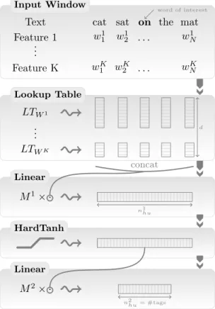
Our architecture is summarized in Figure 1 and Figure 2. The first layer extracts features for each word. The second layer extracts features from a window of words or from the whole sentence, treating it as asequencewith local and global structure (i.e., it is not treated like a bag of words). The following layers are classical NN layers.
3.1 Transforming Words into Feature Vectors
One of the essential keypoints of our architecture is its ability to perform well with the sole use of raw words, without any engineered features. The ability for our method to learn good word representations is thus crucial to our approach. For efficiency, words are fed to our architecture as indices taken from a finite dictionaryD. Obviously, a simple index does
Input Window
Lookup Table
Linear
HardTanh
Linear
Text cat sat on the mat
Feature 1 w1
1 w21 . . . wN1
.. .
Feature K w1K wK2 . . . wKN
LTW1 .. .
LTWK
M1× ·
M2× ·
word of interest
d
concat
n1hu
n2hu= #tags
Figure 1: Window approach network.
not carry much useful information about the word. However, the first layer of our network maps each of these word indices into a feature vector, by a lookup table operation. Given a task of interest, a relevant representation of each word is then given by the corresponding lookup table feature vector, which is trained by backpropagation.
More formally, for each word w ∈ D, an internal dwrd-dimensional feature vector
representation is given by thelookup table layer LTW(·):
LTW(w) =W·w,
whereW ∈Rdwrd×|D|is a matrix of parameters to belearnt,W·
w∈Rdwrd is thewthcolumn
ofW anddwrd is the word vector size (a hyper-parameter to be chosen by the user). Given
a sentence or any sequence of T words [w]T1 in D, the lookup table layer applies the same operation for each word in the sequence, producing the following output matrix:
LTW([w]T1) = W·[w]1 W·[w]2 . . . W·[w]T
. (1)
This matrix can be then fed to further neural network layers, as we will see below.
3.1.1 Extending to Any Discrete Features
One might want to provide features other than words if these features are suspected to be helpful for the task of interest. For example, for the NER task, one could provide a feature
Input Sentence
Lookup Table
Convolution
Max Over Time
Linear
HardTanh
Linear
Text The cat sat on the mat
Feature 1 w1
1 w21 . . . wN1
.. .
Feature K wK
1 wK2 . . . wKN
LTW1 .. .
LTWK
max(·)
M2× ·
M3× ·
d
Padding Padding
n1hu
M1× ·
n1hu
n2hu
n3hu= #tags
Figure 2: Sentence approach network.
which says if a word is in a gazetteer or not. Another common practice is to introduce some basic pre-processing, such as word-stemming or dealing with upper and lower case. In this latter option, the word would be then represented by three discrete features: its lower case stemmed root, its lower case ending, and a capitalization feature.
Generally speaking, we can consider a word as represented by K discrete features w∈ D1× · · · × DK, whereDkis the dictionary for thekthfeature. We associate to each feature a
lookup tableLTWk(·), with parametersWk∈Rd k
wrd×|Dk|wheredk
vector size. Given a wordw, a feature vector of dimensiondwrd=Pkdkwrdis then obtained
by concatenating all lookup table outputs:
LTW1,...,WK(w) =
LTW1(w1) .. . LTWK(wK)
=
Ww11 .. . WwK
K
.
The matrix output of the lookup table layer for a sequence of words [w]T1 is then similar to (1), but where extra rows have been added for each discrete feature:
LTW1,...,WK([w]T1) =
W[1w
1]1 . . . W
1 [w1]T
..
. ...
W[Kw
K]1 . . . W
K [wK]T
. (2)
These vector features learnt by the lookup table learn features for words. Now, we want to use these trainable features as input to further layers of trainable feature extractors, that can represent groups of words and then finally sentences.
3.2 Extracting Higher Level Features from Word Feature Vectors
Feature vectors produced by the lookup table layer need to be combined in subsequent layers of the neural network to produce a tag decision for each word in the sentence. Producing tags for each element in variable length sequences (here, a sentence is a sequence of words) is a classical problem in machine-learning. We consider two common approaches which tag one word at the time: a window approach, and a (convolutional) sentence approach.
3.2.1 Window Approach
A window approach assumes the tag of a word depends mainly on its neighboring words. Given a word to tag, we consider a fixed-sizeksz(hyper-parameter) window of words around
this word. Each word in the window is first passed through the lookup table layer (1) or (2), producing a matrix of word features of fixed size dwrd×ksz. This matrix can be viewed
as adwrdksz-dimensional vector by concatenating each column vector, which can be fed to
further neural network layers.
More formally, we denote zl to be the output of the lth layer of our neural network and adopt the notation h·idwin
t for designating the dwin concatenated column vectors of a
given matrix around thetthcolumn vector. Then, considering thetthword to tag, the word
feature window is:
z1 =hLTW([w]T1i dwin t =
W·[w]t−
dwin/2 .. . W·[w]t
.. . W·[w]t+dwin/2
. (3)
The fixed size vector z1 can be fed to one or several classical neural network layers which perform affine transformations over their inputs:
whereMl∈Rn
l hu×n
l−1
hu andbl ∈Rnlhuare the parameters to betrained. The hyper-parameter
nlhu is usually called thenumber of hidden units of the lth layer.
Several of these layers are often stacked, to extract highly non-linear features. If thelth classical layer is not the last layer, a non-linearity function must follow, or our network would be a simple linear model. We chose a “hard” version of the hyperbolic tangent version, which has the advantage of being slightly cheaper to compute while leaving the generalization performance unchanged.
HardTanh(x) =
−1 ifx <−1
x if −1<=x <= 1 1 ifx >1
. (5)
Finally, the output size of the last layer L of our network is equal to the number of possible tags for the task of interest. Each output can be then interpreted as a score of the corresponding tag (given the input of the network), thanks to a carefuly chosen cost function that we will describe later in this section.
Remark 1 (Border Effects) The feature window (3) is not well defined for words near the beginning or the end of a sentence. To circumvent this problem, we augment the sentence with a special “PADDING” word replicated dwin/2 times at the beginning and the end.
3.2.2 Sentence Approach
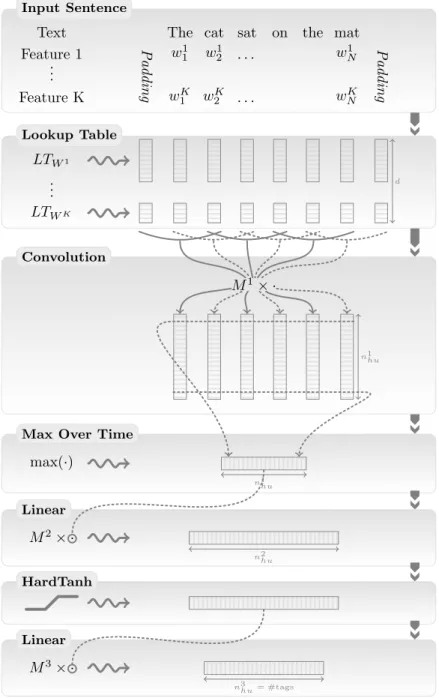
We will see in the experimental section that a window approach performs well for most natural language processing tasks we are interested in. However this approach fails with SRL, where the tag of a word depends on a verb (or, more correctly, predicate) chosen beforehand in the sentence: if the verb falls outside the window, one cannot expect this word to be tagged correctly. In this particular case, tagging a word requires the consideration of thewhole sentence. When using neural networks, the natural choice to tackle this problem becomes a convolutional approach, first introduced by Waibel et al. (1989) and also called Time Delay Neural Networks (TDNNs) in the literature.
We describe in details our convolutional network below. It successively takes the complete sentence, passes it through the lookup table layer (1), produces local features around each word of the sentence thanks to convolutional layers, combines these feature into a global feature vector which can be then fed to classical affine layers (4). In the semantic role labeling case, this operation is performed for each word in the sentence, and for each verb in the sentence. It is thus necessary to encode in the network architecture which verb we are considering in the sentence, and which word we want to tag. For that purpose, each word at position i in the sentence is augmented with two features in the way described in Section 3.1.1. These features encode the relative distances i−posv and
i−posw with respect to the chosen verb at positionposv, and the word to tag at position
posw respectively.
A convolutional layer can be seen as a generalization of a window approach: given a sequence represented by columns in a matrix Zl−1 (in our the lookup table matrix (1)), a matrix-vector operation as in (4) is applied to each window of successive windows in the sequence. Using previous notations, thetth output column of thelthlayer can be computed
as:
Z·lt=MlhZl −1idwin
t +bl, (6)
where the weight matrixMlis the same across all windowstin the sequence. Convolutional layers extract local features around each window of the given sequence. As for classical affine layers (4), convolutional layers are often stacked to extract higher level features. In this case, each layer must be followed by a non-linearity (5) or the network would be equivalent to one convolutional layer.
The size of the output (6) depends on the number of words in the sentence fed to the network. Local feature vectors extracted by the convolutional layers have to be combined to obtain a global feature vector, with a fixed-size independent of the sentence length, in order to apply subsequent classical affine layers. Traditional convolutional networks often apply an average (possibly weighted) or a max operation over the “time” t of the sequence (6). (Here, “time” just means the position in the sentence, this term stems from the use of convolutional layers in e.g. speech data where the sequence occurs over time.) The average operation does not make much sense in our case, as in general most words in the sentence do not have any influence on the semantic role of a given word to tag. Instead, we used a max approach, which forces the network to capture the most useful local features for the task at hand that are produced by the convolutional layers:
zil= max
t Z l−1
i, t 1≤i≤n l−1
hu . (7)
This fixed-sized global feature vector can be then fed to classical affine network layers (4). As in the window approach, we then finally produce one score per possible tag for the given task.
Remark 2 The same border effects arise in the convolution operation (6) as in the window approach (3). We again work around this problem by padding the sentences with a special word.
3.2.3 Tagging Schemes
As explained earlier, the network output layers compute scores for all the possible tags for the task of interest. In the window approach, these tags apply to the word located in the center of the window. In the (convolutional) sentence approach, these tags apply to the word designated by additional markers in the network input.
The POS task consists indeed of marking the syntactic role of each word. However, the remaining three tasks associate tags with segments of a sentence. This is usually achieved by using special tagging schemes to identify the segment boundaries. Several such schemes have been defined (IOB, IOB2, IOE, IOBES, . . . ) without clear conclusion as to which scheme is better in general. State-of-the-art performance is sometimes obtained by combining classifiers trained with different tagging schemes (e.g. Kudo and Matsumoto, 2001).
The ground truth for the NER, CHUNK, and SRL tasks is provided using two different tagging schemes. In order to eliminate this additional source of variations, we have decided to use the most expressive IOBES tagging scheme for all tasks. For instance, in the CHUNK task, we describe noun phrases using four different tags. Tag “S-NP” is used to mark a noun phrase containing a single word. Otherwise tags “B-NP”, “I-NP”, and “E-NP” are used
to mark the first, intermediate and last words of the noun phrase. An additional tag “O” marks words that are not members of a chunk. During testing, these tags are then converted to the original IOB tagging scheme and fed to the standard performance evaluation script.
3.3 Training
All our neural networks are trained by maximizing a likelihood over the training data, using stochastic gradient ascent. If we denoteθto be all the trainable parameters of the network, which are trained using a training setT we want to maximize:
θ7→ X (x, y)∈T
logp(y|x,θ), (8)
where x corresponds to either a training word window or a sentence and its associated features, andyrepresents the corresponding tag. The probabilityp(·) is computed from the outputs of the neural network. We will see in this section two ways of interpreting neural network outputs as probabilities.
3.3.1 Isolated Tag Criterion
In this approach, each word in a sentence is considered independently. Given an input example x, the network with parameters θ outputs a score that we denote f(x, i,θ), for theithtag with respect to the task of interest. This score can be interpreted as a conditional tag probability p(i|x,θ) by applying a softmax (Bridle, 1990) operation over all the tags:
p(i|x,θ) = e
f(x, i,θ)
P
jef(x, j,θ)
. (9)
Defining the log-add operation as logadd
i
zi = log(
X
i
ezi), (10)
we can express the log-likelihood for one training example (x, y) as follows: logp(y|x,θ) =f(x, y, θ)−logadd
j
f(x, j, θ). (11)
While this training criterion, often referred ascross-entropy is widely used for classification problems, it might not be ideal in our case, where often there is a correlation between the tag of a word in a sentence and its neighboring tags. We now describe another common approach for neural networks which enforces dependencies between the predicted tags in a sentence.
3.3.2 Sentence Tag Criterion
In tasks like chunking, NER or SRL we know that there are dependencies between word tags in a sentence: not only are tags organized in chunks, but some tags cannot follow other tags. Training using an isolated tag approach discards this kind of labeling information. We
consider a training scheme which takes in account the sentence structure: given predictions for all tags by our network for all words in a sentence, and given a score for going from one tag to another tag, we want to encourage valid paths of tags during training, while discouraging all other paths.
We define f([x]T1, i, t, θ), the score output by the network with parameters θ, for the sentence [x]T1 and for the ith tag, at the tth word. We introduce a transition scoreAij for
jumping from itoj tags in successive words, and an initial scoreAi0 for starting from the
ith tag. As the transition scores are going to be trained (as are all network parametersθ), we define ˜θ=θ∪ {Aij ∀i, j}. The score of a sentence [x]T1 along a path of tags [i]T1 is then
given by the sum of transition scores and network scores:
s([x]T1,[i]T1,θ˜) =
T
X
t=1
A[i]t−1[i]t+f([x]T1,[i]t, t, θ)
. (12)
Exactly as for the isolated tag criterion (11) where we were normalizing with respect to all tags using a softmax (9), this score can be interpreted as a conditionaltag path probability, by applying a softmax over all possible tag paths [j]T1. Taking the log, the conditional probability of the true path [y]T1 is given by:
logp([y]T1 |[x]T1,θ˜) =s([x]T1,[y]T1,θ˜)−logadd ∀[j]T
1
s([x]T1,[j]T1,θ˜). (13) While the number of terms in the logadd operation (11) was equal to the number of tags, it grows exponentialy with the length of the sentence in (13). Fortunately, one can compute it in linear time with the following classical recursion over t, taking advantage of the associativity and distributivity on the semi-ring4 (R∪ {−∞},logadd,+):
δt(k) ∆
= logadd
{[j]t
1∩[j]t=k}
s([x]t1,[j]t1,θ˜) = logadd
i
logadd {[j]t1∩[j]t−1=i∩[j]t=k}
s([x]t1,[j]t1−1,θ˜) +A[j]t−1k+f([x]t1, k, t, θ)
= logadd
i
δt−1(i) +Aik+f([x]t1, k, t, θ)
=f([x]t1, k, t, θ) + logadd
i
(δt−1(i) +Aik) ∀k ,
(14)
followed by the termination logadd
∀[j]T 1
s([x]T1,[j]T1,θ˜) = logadd
i
δT(i). (15)
We can now maximize in (8) the log-likelihood (13) over all the training pairs ([x]T1,[y]T1). At inference time, given a sentence [x]T1 to tag, we have to find the best tag path which minimizes the sentence score (12). In other word, we must find
argmax
[j]T 1
s([x]T1,[j]T1,θ˜). (16)
The Viterbi algorithm is the natural choice for this inference. It corresponds to performing the recursion (14) and (15), but where the logadd is replaced by a max, and then tracking back the optimal path through each max.
Remark 3 (Graph Transformers) Our approach is a particular case of the discrimina-tive forward training for graph transformers (Bottou et al., 1997; Le Cun et al., 1998). The log-likelihood (13) can be viewed as the difference between the forward score constrained over the valid paths (in our case there is only the labeled path) and the unconstrained forward score (15).
Remark 4 (Conditional Random Fields) Conditional Random Fields (CRFs) (Laf-ferty et al., 2001) over temporal sequences maximize the same likelihood as (13). The CRF model is however linear (which would correspond in our case to a linear neural network). CRFs have been widely used in the NLP world, such as for POS tagging (Lafferty et al., 2001), chunking (Sha and Pereira, 2003), NER (McCallum and Li, 2003) or SRL (Cohn and Blunsom, 2005). Compared to CRFs approaches, we take advantage of our deep network to trainappropriate features for each task of interest.
3.3.3 Stochastic Gradient
Maximizing (8) with stochastic gradient (Bottou, 1991) is achieved by iteratively selecting a random example (x, y) and making a gradient step:
θ←−θ+λ∂logp(y|x,θ)
∂θ , (17)
whereλis a chosen learning rate. Our neural networks described in Figure 1 and Figure 2 are a succession of layers that correspond to successive composition of functions. The neural network is finally composed with the isolated tag criterion (11), or successively composed in the recursion (14) if using the sentence criterion (13). Thus, an analytical formulation of the derivative (17) can be computed, by applying the differentiation chain rule through the network, and through the isolated word criterion (11) or through the recurrence (14).
Remark 5 (Differentiability) Our cost functions are differentiable almost everywhere. Nondifferentiable points arise because we use a “hard” transfer function (5) and because we use a “max” layer (7) in the sentence approach network. Fortunately, stochastic gradient still converges to a meaningful local minimum despite such minor differentiability problems (Bottou, 1991).
Remark 6 (Modular Approach) The well known “back-propagation” algorithm (LeCun, 1985; Rumelhart et al., 1986) computes gradients using the chain rule. The chain rule can also be used in a modular implementation.5 Our modules correspond to the boxes in Figure 1 and Figure 2. Given derivatives with respect to its outputs, each module can independently compute derivatives with respect to its inputs and with respect to its trainable parameters, as proposed by Bottou and Gallinari (1991). This allows us to easily build variants of our networks.
Approach POS Chunking NER SRL
(PWA) (F1) (F1) (F1)
Benchmark Systems 97.24 94.29 89.31 77.92
NN+ITC 96.31 89.13 79.53 55.40
NN+STC 96.37 90.33 81.47 70.99
Table 3: Comparison in generalization performance of benchmark NLP systems with our neural network (NN) approach, on POS, chunking, NER and SRL tasks. We report results with both the isolated tag criterion (ITC) and the sentence tag criterion (STC). Generalization performance is reported in per-word accuracy rate (PWA) for POS and F1 score for other tasks.
Task Window/Conv. size Word dim. Caps dim. Hidden units Learning rate
POS dwin = 5 d0 = 50 d1= 5 n1hu= 300 λ= 0.01
CHUNK ” ” ” ” ”
NER ” ” ” ” ”
SRL ” ” ” n
1
hu= 300
n2
hu= 500
”
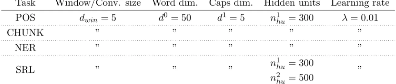
Table 4: Hyper-parameters of our networks. We report for each task the window size (or convolution size), word feature dimension, capital feature dimension, number of hidden units and learning rate.
Remark 7 (Tricks) Many tricks have been reported for training neural networks (LeCun et al., 1998), and it is often confusing which one to choose. We employed only two of them: (1) the initialization of the parameters was done according to the fan-in, and (2) the learning rate was divided by the fan-in (Plaut and Hinton, 1987), but stayed fixed during the training.
3.4 Supervised Benchmark Results
For POS, chunking and NER tasks, we report results with the window architecture described in Section 3.2.1. The SRL task was trained using the sentence approach (Section 3.2.2). Results are reported in Table 3, in per-word accuracy (PWA) for POS, and F1 score for all the other tasks. We performed experiments both with the isolated tag criterion (ITC) and with the sentence tag criterion (STC). The hyper-parameters of our networks are reported in Table 4. All our networks were fed with two raw text features: lower case words, and a capital letter feature. We chose to consider lower case words to limit the number of words in the dictionary. However, to keep some upper case information lost by this transformation, we added a “caps” feature which tells if each word was in low caps, was all caps, had first letter capital, or had one capital. Additionally, all occurences of sequences of numbers within a word are replaced with the string “NUMBER”, so for example both the words “PS1” and “PS2” would map to the single word “psNUMBER”. We used a dictionary
france jesus xbox reddish scratched megabits
454 1973 6909 11724 29869 87025
persuade thickets decadent widescreen odd ppa
faw savary divo antica anchieta uddin
blackstock sympathetic verus shabby emigration biologically
giorgi jfk oxide awe marking kayak
shaheed khwarazm urbina thud heuer mclarens
rumelia stationery epos occupant sambhaji gladwin
planum ilias eglinton revised worshippers centrally
goa’uld gsNUMBER edging leavened ritsuko indonesia
collation operator frg pandionidae lifeless moneo
bacha w.j. namsos shirt mahan nilgiris
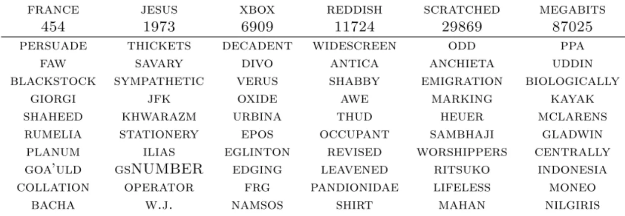
Table 5: Word embeddings in the word lookup table of a SRL neural network trained from scratch, with a dictionary of size 100,000. For each column the queried word is followed by its index in the dictionary (higher means more rare) and its 10 nearest neighbors (arbitrary using the Euclidean metric).
containing the 100,000 most common words in WSJ (case insensitive). Words outside this dictionary were replaced by a single special “RARE” word.
Results show that neural networks “out-of-the-box” are behind baseline benchmark systems. Looking at all submitted systems reported on each CoNLL challenge website showed us our networks performance are nevertheless in the performance ballpark of existing approaches. The training criterion which takes into account the sentence structure seems to always boost the performance for all tasks.
The capacity of our network architectures lies mainly in the word lookup table, which contains 50×100,000 parameters to train. In the WSJ data, 15% of the most common words appear about 90% of the time. Many words appear only a few times. It is thus hopeless to train properly their corresponding 50 dimensional feature vectors in the lookup table. Ideally, we would like semantically similar words to be close in the embedding space represented by the word lookup table: by continuity of the neural network function, tags produced on semantically similar sentences would be identical. We show in Table 5 that it is not the case: neighboring words in the embedding space do not seem to be semantically related.
We will focus in the next section on improving these word embeddings by leveraging unlabeled data. We will see our approach results in a performance boost for all tasks.
Remark 8 (Architectures) We have only tried a few different architectures by validation. In practice, the choice of hyperparameters such as the number of hidden units, provided they are large enough, has a limited impact on the generalization performance.
4. Lots of Unlabeled Data
We would like to obtain word embeddings carrying more syntactic and semantic information than shown in Table 5. Since most of the trainable parameters of our system are associated with the word embeddings, these poor results suggest that we should use considerably more training data. Following our NLP from scratch philosophy, we now describe how to dramatically improve these embeddings using very large unlabeled datasets. We then use these improved embeddings to initialize the word lookup tables of the networks described in Section 3.4.
4.1 Datasets
Our first English corpus is the entire English Wikipedia.6 We have removed all paragraphs containing non-roman characters and all MediaWiki markups. The resulting text was tokenized using the Penn Treebank tokenizer script.7 The resulting dataset contains about 631 million words. As in our previous experiments, we use a dictionary containing the 100,000 most common words in WSJ, with the same processing of capitals and numbers. Again, words outside the dictionary were replaced by the special “RARE” word.
Our second English corpus is composed by adding an extra 221 million words extracted from the Reuters RCV1 (Lewis et al., 2004) dataset.8 We also extended the dictionary to 130,000 words by adding the 30,000 most common words in Reuters. This is useful in order to determine whether improvements can be achieved by further increasing the unlabeled dataset size.
4.2 Ranking Criterion versus Entropy Criterion
We used these unlabeled datasets to trainlanguage models that computescores describing the acceptability of a piece of text. These language models are again large neural networks using the window approach described in Section 3.2.1 and in Figure 1. As in the previous section, most of the trainable parameters are located in the lookup tables.
Very similar language models were already proposed by Bengio and Ducharme (2001) and Schwenk and Gauvain (2002). Their goal was to estimate theprobability of a word given the previous words in a sentence. Estimating conditional probabilities suggests a cross-entropy criterion similar to those described in Section 3.3.1. Because the dictionary size is large, computing the normalization term can be extremely demanding, and sophisticated approximations are required. More importantly for us, neither work leads to significant word embeddings being reported.
Shannon (1951) has estimated the entropy of the English language between 0.6 and 1.3 bits per character by asking human subjects to guess upcoming characters. Cover and King (1978) give a lower bound of 1.25 bits per character using a subtle gambling approach. Meanwhile, using a simple word trigram model, Brown et al. (1992) reach 1.75 bits per character. Teahan and Cleary (1996) obtain entropies as low as 1.46 bits per character using variable length character n-grams. The human subjects rely of course on all their
6. Available athttp://download.wikimedia.org.
7. Available athttp://www.cis.upenn.edu/∼treebank/tokenization.html. 8. Now available athttp://trec.nist.gov/data/reuters/reuters.html.
knowledge of the language and of the world. Can we learn the grammatical structure of the English language and the nature of the world by leveraging the 0.2 bits per character that separate human subjects from simple n-gram models? Since such tasks certainly require high capacity models, obtaining sufficiently small confidence intervals on the test set entropy may require prohibitively large training sets.9 The entropy criterion lacks dynamical range because its numerical value is largely determined by the most frequent phrases. In order to learn syntax, rare but legal phrases are no less significant than common phrases.
It is therefore desirable to define alternative training criteria. We propose here to use a pairwise ranking approach (Cohen et al., 1998). We seek a network that computes a higher score when given a legal phrase than when given an incorrect phrase. Because the ranking literature often deals with information retrieval applications, many authors define complex ranking criteria that give more weight to the ordering of the best ranking instances (see Burges et al., 2007; Cl´emen¸con and Vayatis, 2007). However, in our case, we do not want to emphasize the most common phrase over the rare but legal phrases. Therefore we use a simple pairwise criterion. Let f(s, θ) denote the score computed by our neural network with parametersθ, we minimize the ranking criterion:
θ7→X s∈S
X
w∈D
maxn0, 1−f(s,θ) +f(s(w),θ)o, (18)
where S is the set of text windows coming from our training corpus, D is the dictionary of words, ands(w) denotes the text window obtained by replacing the central word of text
window sby the wordw.
Okanohara and Tsujii (2007) use a related approach to avoiding the entropy criteria using a binary classification approach (correct/incorrect phrase). Their work focuses on using a kernel classifier, and not on learning word embeddings as we do here.
4.3 Training Language Models
The language model network was trained by stochastic gradient minimization of the ranking criterion (18), sampling a sentence-word pair (s, w) at each iteration.
Since training times for such large scale systems are counted in weeks, it is not feasible to try many combinations of hyperparameters. It also makes sense to speedup the training time by initializing new networks with the embeddings computed by earlier networks. In particular, we found it expedient to train a succession of networks using increasingly large dictionaries, each network being initialized with the embeddings of the previous network. Successive dictionary sizes and switching times are chosen arbitrarily. (Bengio et al., 2009) provides a more detailed discussion of this the (as yet, poorly understood) “curriculum” process.
By analogy with biological cell lines, we have bred a few network lines. Within each line, child networks were initialized with the embeddings of their parents and trained on increasingly rich datasets with sometimes different parameters. Breeding decisions were made on the basis of the value of the ranking criterion (18) estimated on a validation set composed of one million words held out from the Wikipedia corpus.
9. However, Klein and Manning (2002) describe a rare example of realistic unsupervised grammar induction using a cross-entropy approach on binary-branching parsing trees, that is, by forcing the system to generate a hierarchical representation.
france jesus xbox reddish scratched megabits
454 1973 6909 11724 29869 87025
austria god amiga greenish nailed octets
belgium sati playstation bluish smashed mb/s
germany christ msx pinkish punched bit/s
italy satan ipod purplish popped baud
greece kali sega brownish crimped carats
sweden indra psNUMBER greyish scraped kbit/s
norway vishnu hd grayish screwed megahertz
europe ananda dreamcast whitish sectioned megapixels
hungary parvati geforce silvery slashed gbit/s
switzerland grace capcom yellowish ripped amperes
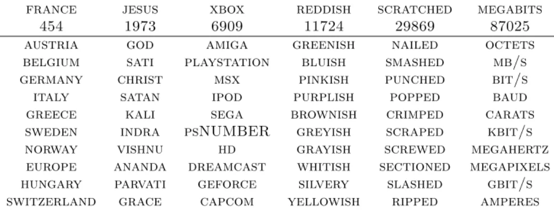
Table 6: Word embeddings in the word lookup table of the language model neural network LM1 trained with a dictionary of size 100,000. For each column the queried word is followed by its index in the dictionary (higher means more rare) and its 10 nearest neighbors (using the Euclidean metric, which was chosen arbitrarily).
Very long training times make such strategies necessary for the foreseable future: if we had been given computers ten times faster, we probably would have found uses for datasets ten times bigger. Of course this process makes very difficult to characterize the learning procedure. However we can characterize the final product.
In the following subsections, we report results obtained with two trained language models. The results achieved by these two models are representative of those achieved by networks trained on the full corpuses.
• Language model LM1 has a window sizedwin = 11 and a hidden layer withn1hu= 100
units. The embedding layers were dimensioned like those of the supervised networks (Table 4). Model LM1 was trained on our first English corpus (Wikipedia) using successive dictionaries composed of the 5000, 10,000, 30,000, 50,000 and finally 100,000 most common WSJ words. The total training time was about four weeks.
• Language model LM2 has the same dimensions. It was initialized with the embeddings of LM1, and trained for an additional three weeks on our second English corpus (Wikipedia+Reuters) using a dictionary size of 130,000 words.
4.4 Embeddings
Both networks produce much more appealing word embeddings than in Section 3.4. Table 6 shows the ten nearest neighbours of a few randomly chosen query words for the LM1 model. The syntactic and semantic properties of the neighbours are clearly related to those of the query word. These results are far more satisfactory than those reported in Table 6 for embeddings obtained using purely supervised training of the benchmark NLP tasks.
Approach POS CHUNK NER SRL
(PWA) (F1) (F1) (F1)
Benchmark Systems 97.24 94.29 89.31 77.92
NN+ITC 96.31 89.13 79.53 55.40
NN+STC 96.37 90.33 81.47 70.99
NN+ITC+LM1 97.05 91.91 85.68 58.18
NN+STC+LM1 97.10 93.65 87.58 73.84
NN+ITC+LM2 97.14 92.04 86.96 58.34
NN+STC+LM2 97.20 93.63 88.67 74.15
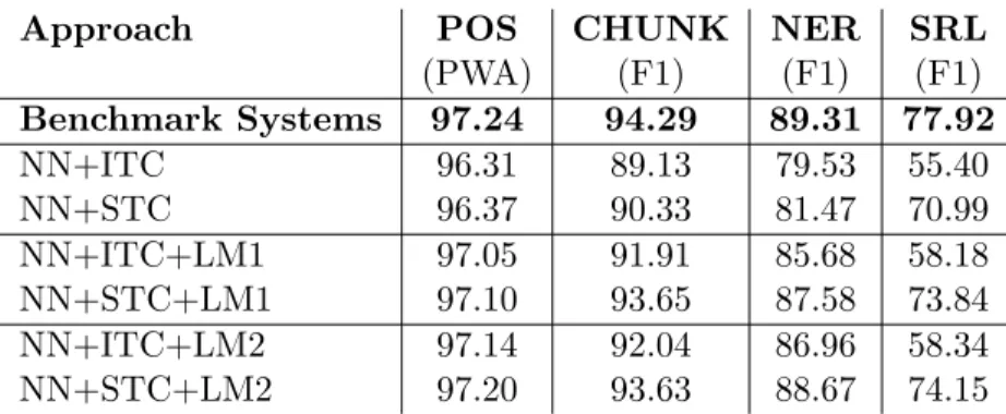
Table 7: Comparison in generalization performance of benchmark NLP systems with our neural network (NN) approach on POS, chunking, NER and SRL tasks. We report results with both the isolated tag criterion (ITC) and the sentence tag criterion (STC). We report with (LMn) performance of the networks trained from the language model embeddings (Table 6). Generalization performance is reported in per-word accuracy (PWA) for POS and F1 score for other tasks.
4.5 Semi-supervised Benchmark Results
Semi-supervised learning has been the object of much attention during the last few years (see Chapelle et al., 2006). Previous semi-supervised approaches for NLP can be roughly categorized as follows:
• Ad-hoc approaches such as (Rosenfeld and Feldman, 2007) for relation extraction.
• Self-training approaches, such as (Ueffing et al., 2007) for machine translation, and (McClosky et al., 2006) for parsing. These methods augment the labeled training set with examples from the unlabeled dataset using the labels predicted by the model itself. Transductive approaches, such as (Joachims, 1999) for text classification can be viewed as a refined form of self-training.
• Parameter sharing approaches such as (Ando and Zhang, 2005). Ando and Zhang propose a multi-task approach where they jointly train models sharing certain parameters. They train POS and NER models together with a language model consisting of predicting words given the surrounding tokens. This work should be seen as a linear counterpart of our approach. Using multilayer models vastly expands the parameter sharing opportunities (see Section 5).
Our approach simply consists of initializing the word lookup tables of the supervised networks with the embeddings computed by the language models. Supervised training is then performed as in section Section 3.4. In particular the supervised training stage is free to modify the lookup tables. This sequential approach is computationally convenient because it separates the lengthy training of the language models from the relatively fast training of the supervised networks. Once the language models are trained, we can perform multiple experiments on the supervised networks in a relatively short time.
Table 7 clearly shows that this simple initialization significantly boosts the generalization performance of the supervised networks for each task. It is worth mentioning the larger
language model led to even better performance. This suggests that we could still take advantage of even bigger unlabeled datasets.
4.6 Ranking and Language
There is a large agreement in the NLP community that syntax is a necessary prerequisite for semantic role labelling (Gildea and Palmer, 2002). This is why state-of-the-art semantic role labelling systems thoroughly exploit multiple parse trees. The parsers themselves (Charniak, 2000; Collins, 1999) contain considerable prior information about syntax.
Our system does not use such parse trees because we attempt to learn this information from the unlabelled data set. It is therefore legitimate to question whether our ranking criterion (18) has the conceptual capability to capture such a rich hierarchical information. At first glance, the ranking task appears unrelated to the induction of probabilistic grammars that underly standard parsing algorithms. The lack of hierarchical representation seems a fatal flaw (Chomsky, 1956).
However, ranking is closely related to a less known mathematical description of the language calledoperator grammars(Harris, 1968). Instead of directly studying the structure of a sentence, Harris studies the structure of the space of all sentences. Starting from a couple of elementary sentence forms, the space of all sentences is described by the successive application of sentence transformation operators. The sentence structure is revealed as a side effect of the successive transformations. Sentence transformations can also have a semantic interpretation.
Following the structural linguistic tradition, Harris describes procedures that leverage statistical properties of the language in order to discover the sentence transformation operators. Such procedures are obviously useful for machine learning approaches. In particular, he proposes a test to decide whether two sentences forms are or are not semantically related by a transformation operator. He first defines a ranking criterion similar to our ranking criterion (Harris, 1968, section 4.1):
“Starting for convenience with very short sentence forms, say ABC, we choose a particular word choice for all the classes, say BqCq, except one, in
this case A; for every pair of members Ai, Aj of that word class we ask how
the sentence formed with one of the members, i.e. AiBqCq compares as to
acceptability with the sentence formed with the other member, i.e. AjBqCq.”
Thesegradings are then used to compare sentence forms:
“It now turns out that, given the graded n-tuples of words for a particular sentence form, we can find other sentences forms of the same word classes in which the samen-tuples of words produce the same grading of sentences.”
This is an indication that these two sentence forms exploit common words with the same syntactical function and possibly the same meaning. This observation forms the empirical basis for the construction of operator grammars that describe real-world natural languages such as English (Harris, 1982).
Therefore there are solid reasons to believe that the ranking criterion (18) has the conceptual potential to capture strong syntactical and semantical information. On the
other hand, the structure of our language models is probably too restrictive for such goals, and our current approach only exploits the word embeddings discovered during training.
5. Multi-Task Learning
It is generally accepted that featurestrainedfor one task can be useful forrelated tasks. This idea was already exploited in the previous section when certain language model features, namely the word embeddings, were used to initialize the supervised networks.
Multi-task learning (MTL) leverages this idea in a more systematic way. Models for all tasks of interests are jointly trained with an additional linkage between their trainable parameters in the hope of improving the generalization error. This linkage can take the form of a regularization term in the joint cost function that biases the models towards common representations. A much simpler approach consists in having the models share certain parameters defined a priori. Multi-task learning has a long history in machine learning and neural networks. Caruana (1997) gives a good overview of these past efforts.
5.1 Joint Decoding versus Joint Training
Multitask approaches do not necessarily involve joint training. For instance, modern speech recognition systems use Bayes rule to combine the outputs of an acoustic model trained on speech data and a language model trained on phonetic or textual corpora (Jelinek, 1976). This joint decoding approach has been successfully applied to structurally more complex NLP tasks. Sutton and McCallum (2005b) obtains improved results by combining the predictions of independently trained CRF models using a joint decoding process at test time that requires more sophisticated probabilistic inference techniques. On the other hand, Sutton and McCallum (2005a) obtain results somewhat below the state-of-the-art using joint decoding for SRL and syntactic parsing. Musillo and Merlo (2006) also describe a negative result at the same joint task.
Joint decoding invariably works by considering additional probabilistic dependency paths between the models. Therefore it defines an implicit supermodel that describes all the tasks in the same probababilistic framework. Separately training a submodel only makes sense when the training data blocks these additional dependency paths (in the sense of d-separation, Pearl, 1988). This implies that, without joint training, the additional dependency paths cannot directly involve unobserved variables. Therefore, the natural idea of discovering common internal representations across tasks requires joint training.
Joint training is relatively straightforward when the training sets for the individual tasks contain the same patterns with different labels. It is then sufficient to train a model that computes multiple outputs for each pattern (Suddarth and Holden, 1991). Using this scheme, Sutton et al. (2007) demonstrates improvements on POS tagging and noun-phrase chunking using jointly trained CRFs. However the joint labelling requirement is a limitation because such data is not often available. Miller et al. (2000) achieves performance improvements by jointly training NER, parsing, and relation extraction in a statistical parsing model. The joint labeling requirement problem was weakened using a predictor to fill in the missing annotations.
Ando and Zhang (2005) propose a setup that works around the joint labeling requirements. They define linear models of the form fi(x) =wi>Φ(x) +vi>ΘΨ(x) where
Lookup Table
Linear
Lookup Table
Linear
HardTanh HardTanh
Linear
Task 1
Linear
Task 2
M2
(t1)× · M
2 (t2)× ·
LTW1 .. .
LTWK
M1× ·
n1hu n1hu
n2hu,(t1)= #tags n2hu,(t2)= #tags
Figure 3: Example of multitasking with NN. Task 1 and Task 2 are two tasks trained with the architecture presented in Figure 1. Lookup tables as well as the first hidden layer are shared. The last layer is task specific. The principle is the same with more than two tasks.
Approach POS CHUNK NER
(PWA) (F1) (F1)
Benchmark Systems 97.24 94.29 89.31
NN+STC+LM2 97.20 93.63 88.67
NN+STC+LM2+MTL 97.22 94.10 88.62
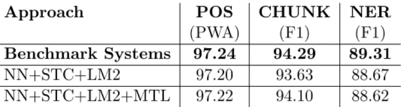
Table 8: Effect of multi-tasking on our neural architectures. We trained POS, CHUNK and NER in a MTL way. As a baseline, we show previous results of our system trained separately on each task. We also report benchmark systems performance for comparison.
fi is the classifier for the i-th task with parameters wi and vi. Notations Φ(x) and Ψ(x)
represent engineered features for the patternx. Matrix Θ maps the Ψ(x) features into a low dimensional subspace common across all tasks. Each task is trained using its own examples without a joint labelling requirement. The learning procedure alternates the optimization of wi and vi for each task, and the optimization of Θ to minimize the average loss for all
examples in all tasks. The authors also consider auxiliary unsupervised tasks for predicting substructures. They report excellent results on several tasks, including POS and NER.
5.2 Multi-Task Benchmark Results
Table 8 reports results obtained by jointly trained models for the POS, CHUNK and NER tasks using the same setup as Section 4.5. All three models share the lookup table parameters (2), and the first hidden layer parameters (4), as illustrated in Figure 3. Best results were obtained by enlarging the first hidden layer size to n1hu = 500 in order to account for its shared responsibilities. The word embedding dimension was kept constant d0= 50 in order to reuse the language models of Section 4.5.
Training was achieved by minimizing the loss averaged across all tasks. This is easily achieved with stochastic gradient by alternatively picking examples for each task and applying (17) to all the parameters of the corresponding model, including the shared parameters. Note that this gives each task equal weight. Since each task uses the training sets described in Table 1, it is worth noticing that examples can come from quite different datasets. The generalization performance for each task was measured using the traditional testing data specified in Table 1. Fortunately, none of the training and test sets overlap across tasks.
Only the chunking task displays a significant performance improvement over the results reported in Section 4.5. The next section shows more directly that this improvement is related to the synergy between the POS and CHUNK task.
6. The Temptation
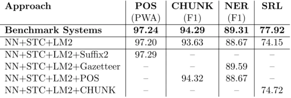
Results so far have been obtained by staying true to ourfrom scratch philosophy. We have so far avoided specializing our architecture for any task, disregarding a lot of usefula priori NLP knowledge. We have shown that, thanks to very large unlabelled datasets, our generic neural networks can still achieve close to state-of-the-art performance by discovering useful features. This section explores what happens when we increase the level of engineering in our systems by incorporating some common techniques from the NLP literature. We often obtain further improvements. These figures are useful to quantify how far we went by leveraging large datasets instead of relying on a priori knowledge.
6.1 Stemming
Word suffixes in many western languages are strong predictors of the syntactic function of the word and therefore can benefit POS system. For instance, Ratnaparkhi (1996) uses inputs representing word suffixes and prefixes up to four characters. We achieve this in the POS task by adding discrete word features (Section 3.1.1) representing the last two characters of every word. The size of the suffix dictionary was 455. This led to a small improvement of the POS performance (Table 9, rowNN+STC+LM2+Suffix2). We also tried suffixes obtained with the Porter (1980) stemmer and obtained the same performance as when using two character suffixes.
6.2 Gazetteers
State-of-the-art NER systems often use a large dictionary containing well known named entities (e.g. Florian et al., 2003). We restricted ourselves to the gazetteer provided by the CoNLL challenge, containing 8,000 locations, person names, organizations, and
Approach POS CHUNK NER SRL
(PWA) (F1) (F1)
Benchmark Systems 97.24 94.29 89.31 77.92
NN+STC+LM2 97.20 93.63 88.67 74.15
NN+STC+LM2+Suffix2 97.29 – – –
NN+STC+LM2+Gazetteer – – 89.59 –
NN+STC+LM2+POS – 94.32 88.67 –
NN+STC+LM2+CHUNK – – – 74.72
Table 9: Comparison in generalization performance of benchmark NLP systems with our neural network (NN) using increasing task-specific engineering tricks. We report as a baseline the previous results obtained with network trained without task-specific tricks. The POS network was trained with two character word suffixes; the NER network was trained using the small CoNLL 2003 gazetteer; the CHUNK and NER networks were trained with additional POS features; and finally, the SRL network was trained with additional CHUNK features.
miscellaneous entities. We trained a NER network with 4 additional word features indicating whether the word is found in the gazetteer under one of these four categories. The resulting system displays a clear performance improvement (Table 9, rowNN+STC+LM2+Gazetteer), establishing a new state-of-the-art NER performance.
6.3 Cascading
When one considers related tasks, it is reasonable to assume that tags obtained for one task can be useful for taking decisions in the other tasks. Conventional NLP systems often use features obtained from the output of other preexisting NLP systems. For instance, Shen and Sarkar (2005) describes a chunking system that uses POS tags as input; Florian et al. (2003) describes a NER system whose inputs include POS and CHUNK tags, as well as the output of two other NER classifiers. State-of-the-art SRL systems exploit parse trees (Gildea and Palmer, 2002; Punyakanok et al., 2005), related to CHUNK tags, and built using POS tags (Charniak, 2000; Collins, 1999).
Table 9 reports results obtained for the CHUNK and NER tasks by adding discrete word features (Section 3.1.1) representing the POS tags. In order to facilitate comparisons, instead of using the more accurate tags from our POS network, we use for each task the POS tags provided by the corresponding CoNLL challenge. We also report results obtained for the SRL task by adding word features representing the CHUNK tags. We consistently obtain moderate improvements.
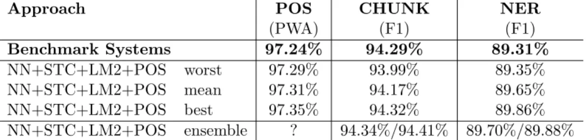
6.4 Ensembles
Constructing ensembles of classifiers is a proven way to trade computational efficiency for generalization performance (Bell et al., 2007). Therefore it is not surprising that many NLP systems achieve state-of-the-art performance by combining the outputs of multiple classifiers. For instance, Kudo and Matsumoto (2001) use an ensemble of classifiers trained
Approach POS CHUNK NER
(PWA) (F1) (F1)
Benchmark Systems 97.24% 94.29% 89.31%
NN+STC+LM2+POS worst 97.29% 93.99% 89.35%
NN+STC+LM2+POS mean 97.31% 94.17% 89.65%
NN+STC+LM2+POS best 97.35% 94.32% 89.86%
NN+STC+LM2+POS ensemble ? 94.34%/94.41% 89.70%/89.88%
Table 10: Comparison in generalization peformance for POS, CHUNK and NER tasks of the networks obtained using by combining ten training runs with different initialization.
with different tagging conventions (see Section 3.2.3). Winning a challenge is of course a legitimate objective. Yet it is often difficult to figure out which ideas are most responsible for the state-of-the-art performance of a large ensemble.
Because neural networks are nonconvex, training runs with different initial parameters usually give different solutions. Table 10 reports results obtained for the CHUNK and NER task after ten training runs with random initial parameters. Simply averaging the predictions of the 10 resulting networks leads to a small improvement over the best network. This improvement comes of course at the expense of a ten fold increase of the running time. On the other hand, multiple training times could be improved using smart sampling strategies (Neal, 1996).
We can also observe that the performance variability is not very large. The local minima found by the training algorithm are usually good local minima, thanks to the oversized parameter space and to the noise induced by the stochastic gradient procedure (LeCun et al., 1998). In order to reduce the variance in our experimental results, we always use the same initial parameters for networks trained on the same task (except of course for the results reported in Table 10.)
6.5 Parsing
Gildea and Palmer (2002) offers several arguments suggesting that syntactical parsing is a necessary prerequisite for the SRL task. The CoNLL 2005 SRL benchmark task provides parse trees computed using both the Charniak (2000) and Collins (1999) parsers. State-of-the-art systems often exploit additional parse trees such as the k top ranking parse trees (Koomen et al., 2005; Haghighi et al., 2005).
In contrast our SRL networks so far do not use parse trees at all. They rely instead on internal representations transferred from a language model trained with an objective function that captures a lot of syntactical information (see Section 4.6). It is therefore legitimate to question whether this approach is an acceptable lightweight replacement for parse trees.
We answer this question by providing parse tree information as input to our system We have limited ourselves to the Charniak parse tree provided with the CoNLL 2005 data. The parse tree information is represented using additional word features encoding the parse tree information at a given depth. We call level 0 the information associated with the leaves
level 0
S NP
The luxury auto maker b-np i-np i-np e-np
NP
last year b-np e-np
VP
sold s-vp
NP
1,214 cars b-np e-np
PP
in s-vp
NP
the U.S. b-np e-np
level 1
S
The luxury auto maker last year
o o o o o o
VP
sold 1,214 cars b-vp i-vp e-vp
PP
in the U.S. b-pp i-pp e-pp
level 2
S
The luxury auto maker last year
o o o o o o
VP
sold 1,214 cars in the U.S. b-vp i-vp i-vp i-vp i-vp e-vp
Figure 4: Charniak parse tree for the sentence“The luxury auto maker last year sold 1,214 cars in the U.S.”. Level 0 is the original tree. Levels 1 to 4 are obtained by successively collapsing terminal tree branches. For each level, words receive tags describing the segment associated with the corresponding leaf. All words receive tag “O” at level 3 in this example.
of the parse tree. We obtain levels 1 to 4 by repeatedly trimming the leaves as shown in Figure 4. Segment boundaries and node labels are encoded using IOBES word tags as discussed in Sections 3.2.3 and 3.1.1.
Experiments were performed using the LM1 language model using the same network architectures (see Table 4) and using additional word features of dimension 5 for each parse tree levels. Table 11 reports the performance improvements obtained by providing increasing levels of parse tree information. Level 0 alone increases the F1 score by almost 1.5%. Additional levels yields diminishing returns. The top performance reaches 76.06% F1 score. This compares nicely with the state-of-the-art system which uses six parse trees instead of one. Koomen et al. (2005) also report a 74.76% F1 score on the validation set using only the Charniak parse tree.
6.6 SENNA: Engineering a Sweet Spot
It is surprising to observe that adding chunking features into the semantic role labelling network (Table 9) performs significantly worse than adding features describing the level 0 of the Charniak parse tree (Table 11). It appears that the parse trees identify leaf sentence segments that are often smaller than those identified by the chunking tags. However we can easily train a second chunking network to identify the segments delimited by the leaves of the Penn Treebank parse trees. We can then retrain the semantic role labelling network using this information as input. Table 12 summarizes the results achieved in this manner.