A VLSI Array Architecture for Hough Transform

A VLSI Array Architecture for Hough Transform

K. Maharatna* Systems Design Dept.

Institute for Semiconductor Physics (IHP)

Technology Park 25, D-15236, Frankfurt (Oder), Germany email: [email protected]

Swapna Banerjee Dept. of E & ECE Indian Institute of Technology Kharagpur – 721302 (INDIA) email: [email protected]

(* Author for correspondence) Abstract:

In this article, an asynchronous array architecture for straight line Hough Transform (HT) is proposed using a scaling free modified CORDIC (Co-Ordinate Rotation Digital Computer) unit as a basic Processing Element (PE). It exhibits four-fold angle parallelism by dividing the Hough space into four subspaces to reduce the computation burden to 25% of the conventional requirements. A distributed accumulator arrangement scheme is adopted to ensure conflict free voting operation. The architecture is then extended to compute circular and elliptic HT given their centers and orientations. Compared to some other existing architectures, this one exhibits higher computation speed.

1. Introduction:

Hough Transform (HT) is a well-known technique for efficient shape recognition(1, 2). High computational complexity and excessive memory requirement are the major obstacles for monolithic integration of HT(3). Memory requirement problem may be simplified by current level of memory integration technique(4).In this paper we restrict ourselves to speed up the computational time of transformation part of the HT i. e., the computation of vote address in the parameter space.

Different architectures and algorithms have been proposed to speed up the computational time for HT(4, 5, 6, 7, 8, 9). Most of the Hough – based methods encounter the evaluation problem of implicit trigonometric and transcendental functions. This makes the monolithic implementation of the entire algorithm rather difficult. To overcome this problem, CORDIC based architectures(3, 10). Are used to generate the vote address in parameter space.

circle), semi major and semi minor radii (for ellipse) as these parameter estimation requires exhaustive arithmetic operations like multiplication, square root evaluation, division, addition / subtraction and squaring(12). To reduce the computation and hardware requirements for the estimation of these parameters, the problems are reformulated in terms of the CORDIC rotation.

The paper has been structured as follows, in Section 2, a brief description of the scaling free modified CORDIC unit is provided. The design of the CORDIC unit is carried out using Transmission Gate Logic (TGL), which shows 62 mW power consumption for 1.6 µm sea of gates technology, that has been described in this Section. In Section 3, theoretical formulation of the straight line HT using an angle parallelization scheme and the corresponding architecture are described. Comparison of this architecture with some other existing architectures is done in Section 4. In Section 5, theoretical formulation for circular and elliptic HT and the corresponding architectures are described. Conclusions are drawn in Section 6.

2. The CORDIC unit:

2.1 Brief description of modified CORDIC unit:

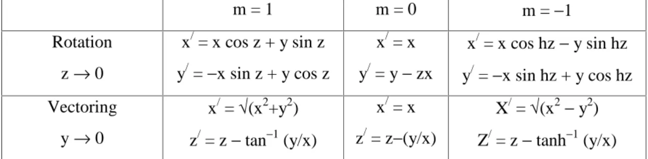
The CORDIC algorithm, first proposed by Volder(13) and unified by Walther(14), is an iterative procedure to compute magnitude and phase or the rotation of a vector in circular, linear and hyperbolic co-ordinate systems, described by the parameter m shown in Table 1.

An initial vector [x y]T undergoing a rotation through an angle ψ, will generate the final vector [x/ y/]T according to the following relation,

The total rotation ψ can be expressed in the steps of smaller angles αi s, such that

∑

ψ (2)

where M is an integer.

Equation (1) can be computed by cascading a number of elementary rotational stages as follows:             − =       ′ ′

∏

i α α

α α cos sin sin cos 1 (3)

If the elementary angles αi are small enough such that sinαi ≅ αi = 2−i and cosαi =

1−2−(2i+1), equation 3 may be written as(11)

              − − − =       ′ ′ + − − − + − =

∏

y x i i i i M

i (2 1(

) 1 2 (

1 2 1 2 2 2

1

(4)

The largest term that we are neglecting in the process of such approximation is αi3/3! = 2−3i/6 = 2−(3i+2.585)

If the machine in which the operations are supposed to be implemented has got an accuracy of b-bits, then multiplying any quantity with αi3/3! will have no effect if

(3i+2.585) equals or exceeds b, that is,

3i+2.585 ≥ b or i ≥ 1/3 (b−2.585)

Since i can adopt only integer values, the above condition essentially becomes

i ≥1/3 (b−2.585)

a 16-bit machine, i ∈ {4, 5, …, 15}. The block diagram of the elementary CORDIC rotor stage i. e., one section corresponding to αi, using this principle is shown in Figure 1. The

detailed description of this modified CORDIC is given in the reference(11). 2.2 Design of the low power CORDIC processor:

A 16-bit CORDIC processor for ψ = 3.583° is designed using the TGL methodology on the sea of gates semicustom design environment. The sea of gates image used here is provided by the OCEAN software (developed in the Delft Technical University, Netherlands). It consists of symmetrically placed fishbone structure constructed by following C3DM (Philips) 1.6 µm double layer CMOS technology. The dimensions of minimum size transistor are 1.6 µm × 23.2 µm (NMOS), 1.6 µm × 29.6

µm (PMOS) having transistor pitch = 8 µm, metal layer width = 2.4 µm (for both metal 1

and metal 2) and the threshold voltage of the devices are 0.7 V (NMOS) and −1.1 V (PMOS)(15).

buffer is not required in TGL and the body effect can be made symmetrical for long TGL chain(16). Since the direct powerline access is not required in TGL style, the static power dissipation due to leakage current is expected to be low. Implementation of the logic circuits using TGL requires less number of transistors than the conventional CMOS design style and thus the area consumption in the former case is lower. Considering these features, the TGL style is selected for our purpose.

The performance of the circuit is analyzed by the Switch Level timing Simulator (SLS) provided with the OCEAN package. The extracted netlist from the layout contains nodal, parasitic and routing capacitance. The design is characterized by its delay, dynamic power consumption, Power-Delay Product (PDP) and Energy-Delay Product (EDP). The dynamic power calculation of the circuit is carried out by conventional dynamic power dissipation formula(16)

∑

= = n i

DD Li iC V f

P

1

2 β

where P is the power consumption, n is the number of internal nodes, βi is the

switching probability of the i th node, CLi is the i th load capacitance, f is the operation

frequency and VDD is the supply voltage. The switching probability is considered as 1 in

order to include the glitching effect which may exhibit the upper limit of worst case power consumption.

The simulated circuit extracted from the layout shows that the worst case delay of the CORDIC processor is 22.72 nsec. At 5 V supply with 44 MHz operation frequency, the dynamic power consumption, PDP and EDP of the CORDIC are 62 mW, 1.408 nJ and 3.2 × 10−17 Jsec. respectively. With proper threshold voltage and device scaling, the supply voltage can be lowered further to achieve quadratic improvement in power performance(16).

3. The straight line HT:

3.1 The mathematical formulation:

The Duda – Hart parameterization for detecting straight lines in an edge image is defined as(17)

ρ θ θ + sin =

cos y

x (5)

where ρ is the normal distance of the straight line from the origin of the co-ordinate system and θ is the angle between the normal and x-axis as shown in Figure 2. The values of θ and ρ are restricted in the intervals [0, π] and [−R, R] respectively. In computing the

transform, the ρ - θ space (often called the parameter space or the Hough space) is quantized in steps of [θi, ρj], where i, j are two integers. The quantized parameter space is

represented by a 2-D accumulator array. The image space points lying on the line defined by equation (5) with the parameters (θi, ρj) will vote to the (θi, ρj) th accumulator cell and

generate a histogram. Extraction of the straight line can be done by considering the accumulator counts above a predefined threshold value.

Equation (5) can be implemented using CORDIC which is evident from equation (1). From equation (1), one gets,

θ

θ sin

cos y

x

θ

θ cos

sin y

x

y′=− + (7)

Equation (6) and (7) show that the CORDIC provides two concurrent outputs with their arguments lying π/2 angle apart.

Now replacing (45° + θ) in place of θ in equations (6) and (7), we have another two equations as follows:

)] cos sin ( ) sin cos [(

2x′′= x θ + y θ + −x θ + y θ (8)

)] sin cos ( ) cos sin [(

2y′′= −x θ + y θ − x θ + y θ (9)

These equations imply that a scan range of θ ∈ [0, π] can be divided into four independent subspaces A (θ ∈ [0°, 45°]), B (θ ∈ [45°, 90°], C (θ ∈ [90°, 135°]) and D (θ ∈ [135°, 180°]). Thus, parallely computing equations (6), (7), (8) and (9) with θ∈ [0°, 45°] covers the whole scan range of θ. This result can be utilized for parallel computation of straight line HT.

Defining ρA, ρB, ρC and ρD as the sets of ρ values in the subspaces A, B, C and D

respectively, four equations can be formulated corresponding to the four subspaces as shown below,

θ θ

ρ_A =xcos + ysin (10)

)] cos sin ( ) sin cos [(

2ρB = x θ + y θ + −x θ + y θ (11)

θ θ

ρC =−xsin + ycos (12)

)] sin cos ( ) cos sin [(

2ρ_D = −x θ + y θ +− x θ + y θ (13) In equations (11) and (13) the term √2 is a constant and can be taken care by look

up table approach or by the addressing logic. Alternatively, √2ρB and √2ρD can be

computed from their modified values after thresholding. Thus, defining ρB/ (=√2ρB) and

ρD/ (=√2ρD) as the modified parameters in the subspaces B and D respectively, one can

rewrite equations (11) and (13) in terms of ρA and ρC as follows,

ρB/ = ρA + ρC (14)

ρD/ = ρC−ρA (15)

Using CORDIC, equations (10) and (13) can be computed concurrently and from this, equations (14) and (15) can also be computed.

3.2 Array architecture for straight line HT:

The array architecture for straight line HT has been constructed by suitable mapping of equations (10), (12), (14) and (15). The entire θ scan range [0, π/4] is quantized into N equal angular segments each having a value θ0 such that,

Nθ0 = π/4 ±δ where δ = 0, if π/4 is an integer multiple of θ0

δ ≠ 0, if π/4 is not an integer multiple of θ0

The basic PE is shown in Figure 3 which is designated as HS. It consists of one CORDIC rotor unit, two adders and four independent accumulator banks: AA, AB, AC and

AD for the storage of ρA, ρB/, ρC and ρD/ values respectively. The CORDIC rotor parallely

generates the addresses of ρA and ρC by computing equations (13) and (15). These two ρ

values are then utilized for parallel address computation of ρB/ and ρD/ using the adders.

computation at different θ (= jθ0, j ∈ {1, 2, …, N}) can be done for N feature points. The

peak detection can be carried out by checking the accumulator counts parallely for all HS. The total architecture is shown in Figure 4. The whole operation is summarized in the following pseudocode,

Let p ∈ {1, 2, …, N} be the index of the PE and q ∈ {1, 2, …, M} be the index of the accumulator array for each PE. θ0 is the rotation introduced by a single processor and

Nθ0 = π/4 ± δ. ρpqA denotes the value of ρ corresponding to the q th accumulator cell in

subspace A for angle pθ0 and so on.

1. ∀ p th PE, initialize the accumulator cell counts to zero.

2. For each edge pixel (x, y) with grey level equal to one, ∀ p th PE, do in parallel

(a) compute in parallel

ρpqA = xp = x(p−1) cosθ0 + y(p−1) sinθ0 = x cos (pθ0) + y sin (pθ0)

ρpqC = yp = − x(p−1) sinθ0 + y(p−1) cosθ0 = − x sin (pθ0) + y cos (pθ0)

(b) compute in parallel ρpqB/ = ρpqA +ρpqC

ρpqD/ = −ρpqA + ρpqC

(c) update q th Hough array in parallel for all the subspaces. (d) Check the busy bit of (p+1) th PE.

if busy bit is high enter in wait state. if busy bit is low

(e) assert busy bit of p th and (p+1) th PE in logic low and high state respectively. (f) get new input.

(g) assert busy bit of p th PE in logic high state.

3. Look for peaks in the accumulator array∀ p.

3.3 Performance of the architecture:

To evaluate the performance of the proposed architecture and to compare it with the other proposed methods we assume that in the proposed one θ space is quantized in step of θ0, where Nθ0 = π/4 ±δ, n be the number of edge pixels to be processed and m be

the number of accumulators per subspace for full set of ρ for each θ0.

3.3.1 Computational complexity:

The total number of operations required for ρ computation using the conventional method is 2nπ/θ0 trigonometric multiplication + nπ/θ0 additions whereas, in the proposed

method, the total arithmetic operations required is 6nπ/4θ0 (=1.5 nπ/θ0) additions which

is much less than the conventional method as the θ scan range is restricted between [0, π/4±δ]. The total accumulator cell requirement in the proposed method is equal mπ/θ0,

which is same as the conventional one. 3.3.2 Area – Time complexity (AT):

Considering the area of one adder be O(a) and the area of one accumulator cell be

O(ac), the area of one PE is O(6a+4mac). Thus, the area consumed by the proposed architecture is

The latency of the proposed architecture is O (π/4θ0) and the time required to

compute the rest (n−1) feature points is O(n−1), where the time required for one PE is taken as O(1). Thus, the total computation time becomes,

T = O [(π/4θ0)+(n−1)] = O[N + (n−1)]

If the time required for an adder is Ta, the total computation time T can be represented as

T = O[2{N + (n−1)}Ta ]

So the AT of the proposed one is equal to O[2N(6a+4mac) {N + (n−1)}Ta ].

4. Comparison with other architectures:

In this section the proposed architecture is compared with some of the existing architectures based on the nature of PE, angle scan range, time requirement for histogram generation and extra hardware requirements. The comparison is carried out by considering the number of θ0 values in the range [0, π/4+δ] to be N, O(Ts) and O(Ta) be

N = 13 and δ = 1.534085° and Ta = 7.1 nsec (in 1.6 µm sea of gates technology). Under

these considerations, a full set of ρ value generation for one feature point takes 295.36 nsec, which seem to be considerably low.

Since this architecture utilizes CORDIC, unlike multiplier based designs, the precomputations of ‘cos’ and ‘sin’ values are not required which in its way eliminates the requirement of RAM. This makes the architecture more time effective compared to the multiplier based designs, as in the later case, the RAM access time become a deterministic constraint for ρ computation as is evident in the reference(4).

In the proposed architecture, the CORDIC units require only adder-subtractor and the architecture can simultaneously compute ρ for N angles in the θ scan range of [0, π/4+δ]. Being composed of the scaling free CORDIC (discussed in Section 2), the

architecture is more hardware efficient compared to the other CORDIC based implementations and does not require the extra conversion unit like the architecture of reference(10).

The distributed accumulator cell arrangement with each PE ensures conflict free voting operation. This facilitates a parallel approach for peak detection by simultaneously checking the count of the accumulators for all θ0, i. e. for all PE.

In light of the above results and discussion, it can be conjectured that this architecture can be considered as a potential candidate for low power high performance real time straight line HT using VLSI.

5. Circular and elliptic HT:

Subsequently, CORDIC based array architectures are proposed for them. Analyses made here are based on two considerations that are,

• The origin of the curves is already known.

• The orientation angle of the ellipse is known.

5.1 Circular HT:

The equation of a circle can be stated as, 2 2 2

r y

x + = (16) where, (x, y) is a point lying on the circle and ‘r’ is the radius. In parametric form the length of the radius is given by,

xcosθ + ysinθ =r (17) where θ is the angle made by the radius vector with the positive x-axis as shown in Figure 5. Equation (17) is exactly similar to equation (5) and thus the same architecture for straight line HT can be extended for circular HT. All the points lying on the same circle will give same radius value for different θ. Considering the co-ordinate system where the origin is coincident with the center of the circle, the θ scan range will be of [0, 2π]. This range can be divided into eight subspaces (a, b, c, d, e, f, g, h) and the θ scan range can be restricted to [0, π/4 ± δ]. The values of r in different subspaces can be calculated according to the following equations,

θ

θ sin

cos y

x

r_a = + (θ∈ [0, 45°±δ]) (18) θ

θ cos

sin y

x

rc =− + (θ ∈ [90°, 135°±δ]) (19)

c a b

b r r r

r = / = +

2 (θ∈ [45°, 90°±δ]) (20)

a c d

d r r r

r = / = −

a

e r

r =− (θ∈ [180°, 225°±δ]) (22) /

b

f r

r =− (θ∈ [225°, 270°±δ]) (23)

c

g r

r =− (θ∈ [270°, 315°±δ]) (24) /

d

h r

r =− (θ∈ [315°, 360°±δ]) (25) Where, the suffix of r defines their values in appropriate subspaces and rb/ and rd/ are

considered as modified parameters in the respective subspaces. It can be observed that only (18) and (19) are needed to be computed which can be readily done using CORDIC. Equations (20) and (21) can be derived from (18) and (19) by simple addition and subtraction. The other four equations can be directly computed by only changing the signs of the equations (18), (19) and (21). Thus, for detecting the radius of circle, the architecture for straight line HT can be used with extra four accumulator arrays for each PE since r-values for eight subspaces are to be stored. Finally, checking the votes of the same indexed accumulator cells for different PE (i. e. for different θ), the radius of the circle can be found out. If the circle has its center at (x0, y0), then in this formulation, x

and y have to be replaced by X = (x−x0) and Y = (y−y0). The basic PE (designate as HC) and the architecture for the circular HT are shown in Figure 6 (a) and (b) respectively. 5.2 Elliptic HT:

The parametric equation of a point (x, y) lying on an ellipse with semi-major and semi-minor radii ‘a’ and ‘b’ respectively, is given by

θ cos

a

x= (26) θ

sin

b

where θ is the angle made by the radius vector (from origin to the (x, y) point) with the positive x-axis.

Now, defining 1/a = a/ and 1/b = b/, equation (26) and (27) can be written as θ

cos ) / 1 ( x

a′= (28) θ

sin ) / 1 ( y

b′= (29) The quantities a/ and b/ can be considered as modified parameters instead of a, b and can be quantized accordingly. Following the same line of mathematical formulation of circular HT, here also the total θ scan range can be restricted to [0, π/4 ±δ] and the whole Hough space of [0, 2π] can be divided into eight subspaces (a, b, c, d, e, f, g, h). The modified parameter values in these subspaces can be computed according to the following equations,

aa/ = (1/x) cosθ and ba/ = (1/y) sinθ (θ∈ [0, 45°±δ]) (30)

ac/ = −(1/x) sinθ and bc/ = (1/y) cosθ (θ∈ [90°, 135°±δ]) (31) √2ab/ = ab// = aa/ + ac/ and √2bb/ = bb// = ba/ + bc/ (θ∈ [45°, 90°±δ]) (32) √2ad/ = ad// = ac/− aa/ and √2bd/ = bd// = bc/− ba/ (θ∈ [135°, 180°±δ]) (33)

ae/ = − aa/ and be/ = − ba/ (θ∈ [180°, 225°±δ]) (34)

af/ = − ab// and bf/ = − bb// (θ∈ [225°, 270°±δ]) (35)

ag/ = − ac/ and bg/ = − bc/ (θ∈ [270°, 315°±δ]) (36)

ah/ = − ad// and bh/ = − bd// (θ∈ [315°, 360°±δ]) (37)

The other four addresses can be computed by changing the sign of the addresses given by equations (30) and (33). Finally, the votes of the same indexed accumulator cells for different PE will determine the shape of the ellipse and the conversion from a/, b/ to a, b can be carried out using a look-up table. However, the nature of equations (32) and (33) suggests that each PE requires two CORDIC units operating parallely. Each PE also requires eight 2-D accumulator arrays of which each one is dedicated for a particular subspace. The basic PE designated as He and the architecture are shown in Figure 7 (a) and (b) respectively.

If the center of the ellipse lies at (x0, y0) point, then in the above formulation the x and y values have to be replaced by X = (x− x0) and Y = (y− y0) respectively.

5.3 Discussions on elliptic and circular HT architecture:

Compared to the conventional method, the proposed formulations require less number of arithmetic operations to detect the radius of the circle and semi-major and semi-minor radii of the ellipse. In evaluating these parameters conventional method requires multiplication, squaring, subtraction, division and square root evaluation(12). In our formulation, only the CORDIC rotation is required which in turn requires only additions and cross-coupled bus connections. Thus, a large area and resource saving is possible. In the proposed architectures concentric circles and ellipses can be found out directly by checking the votes of the accumulator cells with different indices in their respective cases.

6. Conclusions:

precomputations and RAM, making this one hardware and time efficient compared to the multiplier based architectures. Using an angle parallelization scheme the computation burden is reduced to approximately 25 %. Moreover, this one enjoys superiority in processing speed compared to some other architectures.

The architectures proposed in this paper for computing circular and elliptic HT with known centers and orientations require less number of arithmetic operations compared to the conventional formulations. In our formulation, the computation in eight subspaces can be carried out parallely which results into saving of hardware resources and speeds up the computation time. For computation of circular and elliptic Hough transform utilizing the hierarchical method, these architectures can be considered as the subunits of the respective systems. One the other hand, one may compute the less computation intensive stages of the hierarchy viz., centers (for circle and ellipse) and the orientation (for ellipse) using software and then can utilize these array architectures for fast estimation of the radius (for circle) and major and minor radii (for ellipse).

vectorization mode. Though, this problem is not present in straight line and circular HT architectures.

The basic CORDIC unit has been designed using TGL on 1.6 µm sea of gates semicustom environment which exhibits 62 mW power consumption at 5 V supply and 44 MHz operation frequency. With device scaling, this CORDIC unit is expected to operate at lower supply voltage, which implies that a quadratic advantage in power consumption can be achieved.

References

1. P. V. C. Hough, Method and means of for recognizing complex patterns, U. S. Patent 3069654 (1962).

2. K. Y. Huang, K. S. Fu, T. H. Sheen and S. W. Cheng, Image processing of seismograms: (A) Hough transformation for the detection of seismic patterns; (B) thinning process in the seismogram, Pattern Recognition 18, 429 – 440 (1985).

3. D. Timmerman, H. Hahn and B. J. Hosticka, Hough transform using CORDIC method, Electronics Letters 25, 205 0 206 (1989).

4. K. Hanahara, T. Maruyama and T. Uchiyama, A real time processor for the Hough transform, IEEE Trans. PAMI 10, 121 – 125 (1987).

5. H. Y. H. Chuang and C. C. Li, A systolic array processor for straight line detection by modified Hough transform, IEEE Workshop, Comput. Arch. Pattern Analysis

Database Mgmnt., pp. 300 – 303 (1985).

6. H. A. H. Ibrahim, J. R. Kender and D. E. Shaw, The analysis and performance of two middle-level vision tasks on a fine grained SIMD tree machine, Conf. Comput. Vision

Pattern Recognition, 248 – 256 (1985).

7. H. F. Li, D. Pao and R. Jayakumar, Improvements and systolic implementation of the Hough transformation for straight line detection, Pattern Recognition 22, 697 – 706 (1989).

8. F. M. Rhodes et al., A monolithic Hough transform processor based on restructurable VLSI, IEEE Trans. PAMI 10, 106 – 110 (1988).

9. T. M. Silberberg, The Hough transform on the geometric arithmetic parallel processor, IEEE Workshop, Comput. Arch. Pattern Analysis Database Mgmnt., pp. 387 – 393 (1985).

10. J. D. Bruguera, N. Guil, T. Lang, J. Villalba and E. L. Zapata, CORDIC based parallel / pipelined architecture for the Hough transform, VLSIVideo 12, pp. 207 – 221 (1996).

12. H. K. Muammar and M. Nixon, Tristage Hough transform for multiple ellipse extraction, IEE Proc. – E 138, 27 – 35 (1991).

13. J. E. Volder, The CORDIC trigonometric computing technique, IRE Trans.

Electronic Computers EC-8, 330 – 334 (1959).

14. J. S. Walther, A unified algorithm for elementary functions, AFIPS Conf. Proc. 38, 379 – 385 (1971).

15. P. Groeneveld and P. Stravers, OCEAN: The sea-of-gates design system user’s

manual (1993).

16. A. Bellaouar and M. I. Elmasry, Low-Power Digital VLSI Design, Circuits and Systems, Kluwer Academic Publishers, 1995.

Table 1

m = 1 m = 0 m = −1

Rotation z → 0

x/ = x cos z + y sin z y/ = −x sin z + y cos z

x/ = x y/ = y − zx

x/ = x cos hz − y sin hz y/ = −x sin hz + y cos hz Vectoring

y → 0

x/ = √(x2+y2) z/ = z − tan−1 (y/x)

x/ = x z/ = z−(y/x)

X/ = √(x2− y2) Z/ = z − tanh−1 (y/x)

Table 2

Logic family Average output capacitance (fF)

Average Delay (nsec.)

Power dissipation

(mW)

Power Delay Product (pJ)

Energy Delay product (10−21 Jsec.) Static

CMOS 304.106 1.256 1.5329 1.9253 2.4181

Domino

CMOS 192.969 1.35 2.1867 2.9522 3.9854

NMOS pass

logic 42.1623 0.153 0.052 0.007956 0.001217

Table 3

Architecture Nature of PE Scan range of θ Time required to generate

histogram

Extra requirements

Rhodes et al.(8) Multipliers, architecture is

WSI

[0, π] 20 msec.

(image size 256

× 256, 1/10 of the image are edge pixels)

Precomputed values of sinθ, cosθ and RAM

Hanahara et al.(4) Array multipliers and off chip components

[0, π] 256 msec. For 1024 feature

points.

Precomputed values of sinθ, cosθ and RAM

Timmerman et al.(3) Radix-2 conventional CORDIC unit. Effective scan range is [0, π/4]

O[2MNn (TS + Ta)]

Scaling factor compensation. Bruguera et al.(10) Mixed radix pipelined CORDIC

[0, π/2] O[52Ta + 4(n−1) + Tconv]

Scaling factor compensation,

extra conversion unit

and RAM. Proposed Scaling free

CORDIC. The architecture is asynchronous.

[0, π/4 ±δ] O[2{N+(n−1)} Ta] 149.179 µsec for 256 ×256 image and 23.569 µsec for

1024 points.

Scaling of ρ by the constant factor √2 in B

Table Captions

Table 1. The CORDIC arithmetic function.

Table 2. Comparison of different logic families using the XOR structure.

Table 3. Comparison of different architectures for straight line Hough transform.

Figure Captions Figure 1. The elementary CORDIC arithmetic unit. Figure 2. Normal description of the straight line.

Figure 3. The basic PE for straight line Hough transform.

Figure 4. The array architecture for straight line Hough transform. Figure 5. The parametric representation of a circle.

Figure 6 (a). The basic PE for circular Hough transform.

Figure 6 (b). The array architecture for circular Hough transform. Figure 7 (a). The basic PE for elliptic Hough transform.

Authors’ biography

Koushik Maharatna was born in Calcutta, India in the year 1972. He received his

Bachelors degree in Physics in the year 1993 from the University of Calcutta. In 1995 he received Masters degree in Electronics Science from the same University. In 1997 he joined the Ph. D. program under the joint collaboration of Jadavpur University, Calcutta and Indian Institute of Technology, Kharagpur and completed the doctoral work in the year 2000. Currently he is a Post Doctoral fellow in the Institute for Semiconductor Physics, Frankfurt (Oder), Germany. His research interests include digital signal processing, VLSI array architectures and low power circuit realization.

Swapna Banerjee received her B.E. and M.E. degree in Electronics and

+

−

2i+1 bit shifter

i bit shifter

+

+

+

−

+

−

2i+1 bit shifter

i bit shifter x

y

x/

y/

αi x

y

x/ = x cosαi + y sinαi

y/ = −x sinαi + y cosαi

Figure 1

y

x

ρ

θ

θ

A

A

A

A

+ ₊

+ −

x

y

y

p

x

H

x

y

x

y

Figure 3

H

H

H

H

x

y

p

1

2

3

N

r

θ

x

y

θ

+ ₊ + −

x

y

y

p

x

H

x

y

x

y

Figure 6 (a)

H

H

H

H

x

y

p

1

2

3

N

Figure 6 (b)

a b

c d

e f

g h

×

−

1

×

−

1

×

−

1