See All by Looking at A Few:
Sparse Modeling for Finding Representative Objects
Ehsan Elhamifar
Johns Hopkins University
Guillermo Sapiro
University of Minnesota
Ren´e Vidal
Johns Hopkins University
Abstract
We consider the problem of finding a few representatives for a dataset, i.e., a subset of data points that efficiently describes the entire dataset. We assume that each data point can be expressed as a linear combination of the resentatives and formulate the problem of finding the rep-resentatives as a sparse multiple measurement vector prob-lem. In our formulation, both the dictionary and the mea-surements are given by the data matrix, and the unknown sparse codes select the representatives via convex optimiza-tion. In general, we do not assume that the data are low-rank or distributed around cluster centers. When the data do come from a collection of low-rank models, we show that our method automatically selects a few representatives from each low-rank model. We also analyze the geometry of the representatives and discuss their relationship to the vertices of the convex hull of the data. We show that our framework can be extended to detect and reject outliers in datasets, and to efficiently deal with new observations and large datasets. The proposed framework and theoretical foundations are il-lustrated with examples in video summarization and image classification using representatives.
1. Introduction
In many areas of machine learning, computer vision, sig-nal/image processing, and information retrieval, one needs to deal with massive collections of data, such as databases of images, videos, and text documents. This has motivated a lot of work in the area of dimensionality reduction, whose goal is to find compact representations of the data that can save memory and computational time and also improve the performance of algorithms that deal with the data. More-over, dimensionality reduction can also improve our under-standing and interpretation of the data.
Because datasets consist of high-dimensional data, most dimensionality reduction methods aim at reducing the feature-space dimension for all the data, e.g., PCA [25], LLE [34], Isomap [36], Diffusion Maps [7], etc. However, another important problem related to large datasets is to find
a subset of the datathat appropriately represents the whole dataset, thereby reducing theobject-spacedimension. This is of particular importance in summarizing and visualizing large datasets of natural scenes, objects, faces, hyperspec-tral data, videos, and text. In addition, this summarization helps to remove outliers from the data as they are not true representatives of the datasets. Finally, memory require-ment and computational time of classification and cluster-ing algorithms improve by workcluster-ing on a reduced number of representative data as opposed to a large number of data.
Prior Work. To reduce the dimension of the data in the object-space and find representative points, several meth-ods have been proposed [19, 21, 26, 27, 38]. However, most algorithms assume that the data are either distributed around centers or lie in a low-dimensional space. Kme-doids [26], which can be considered as a variant of Kmeans, assumes that the data are distributed around several clus-ter cenclus-ters, called medoids, which are selected from the data. Kmedoids, similar to Kmeans, is an iterative algo-rithm that strongly depends on the initialization. When similarities/dissimilarities between pairs of data are given and there is a natural clustering based on these similarities, Affinity Propagation [19], similar to Kmedoids, tries to find a data center for each cluster using a message passing al-gorithm. When the collection of data points is low-rank, Rank Revealing QR (RRQR) algorithm [5,6] tries to se-lect a few data points by finding a permutation of the data that gives the best conditioned submatrix. The algorithm has suboptimal properties, as it is not guaranteed to find the globally optimal solution in polynomial time, and also re-lies on the low-rankness assumption. In addition, random-ized algorithms for selecting a few columns from a low-rank matrix have been proposed [38]. For a low-rank matrix with missing entries, [2] proposes a greedy algorithm to select a subset of the columns. For a data matrix with nonnegative entries, [17] proposes a nonnegative matrix factorization us-ing an`1/`∞optimization to select some of the columns of the data matrix for one of the factors.
Paper Contributions. In this work, we study the problem of finding data representatives using dimensionality reduc-tion in the object-space. We assume that there is a subset
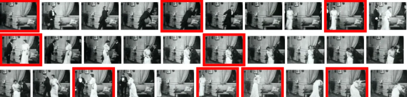
Figure 1.Some frames of the Society Raffles video and the automatically computed representatives of the whole video sequence using our algorithm. The representatives summarize the video as follows: 1) there is a nicely-decorated living room, with a door stage left and a settee in front of an open window in the foreground; 2) a man in the room is talking to someone across the window; 3) a couple enter the room, a man and a woman who is wearing a white gown, and a jeweled tiara. Someone, probably the first man, is standing on the other side of the room; 4) the man who entered with the woman is talking to her and bowing, probably he wants to leave; 5) the first man is sitting with the woman and is reaching for her tiara; 6) the first man is leaving the room, a person is standing across the window and examining the tiara; 7) the woman is entering back to the living room, so she had followed the first man to the door; 8) the woman is clutching her head seeing the bandit across the window; 9) the woman is fainting on the sofa and the bandit has disappeared.
Figure 2.Some frames of a tennis match video, which consists of multiple shots, and the automatically computed representatives of the whole video sequence using our algorithm. Depending on the amount of activities in each shot of the video, we obtained one or a few representatives for that shot.
of data points, called representatives, such that each point in the dataset can be described as a linear combination of a few of the representative points. More specifically, collect-ingN data points of a dataset inRmas columns of a data
matrixY ∈Rm×N, we consider the optimization problem
minkY −Y Ck2F s.t. kCkrow,0≤k, 1>C=1>, (1)
whereC ∈ RN×N is the coefficient matrix andkCk
row,0
counts the number of nonzero rows ofC[24,37]. In other words, we wish to find at mostkN representatives that best reconstruct the data collection. This can be viewed as a sparse dictionary learning scheme [1,30,33] where the atoms of the dictionary are chosen from the data points and, instead of letting the support for the sparse codes be arbi-trary, we enforce them to have a common support.
The self-expressiveness property,Y = Y C, has been studied for subspace clustering using sparse representation [11, 15] and low-rank representation [18, 29]. However, these algorithms are not targeted at finding representatives because of the norms they use forC. A framework simi-lar to that in (1), with a nonnegativity constraint onC and without the affine constraint, has been used for nonnegative matrix factorization for the problem of hyperspectral imag-ing endmember identification [17], without the analysis of the selected columns. In the context of dictionary learning,
[4] and [31] use kCkrow,0 to design compact dictionaries and to select similar patches in an image, respectively.
In this work, we propose an algorithm for solving a con-vex relaxation of (1) and provide an analysis of the theoreti-cal guarantees of the algorithm. Our work has the following contributions with respect to the state of the art:
– Unlike prior works, we do not assume that the data are low-rank or distributed around cluster centers. We only re-quire the total number of representatives to be much smaller than the number of actual points in the dataset.
– When the data come from a collection of low-rank mod-els, we show that our method automatically selects a few data points from each model.
– We analyze the geometry of representatives and show that they correspond to vertices of the convex hull of the data. – We propose a framework to detect and reject outliers from the dataset using the solution of the proposed optimization program. We also show how to deal with new observations and large datasets efficiently.
– We demonstrate the proposed framework in applications to video summarization (Figs. 1-2) and classification using representatives.
2. Problem Formulation
Consider a set of points inRmarranged as the columns
of the data matrix Y =
y1 . . . yN
. In this section, we formulate the problem of finding representative objects from the collection of data points.
2.1. Learning Compact Dictionaries
Finding compact dictionaries to represent data has been well-studied in the literature [1, 16, 25, 30, 33]. More specifically, in dictionary learning problems, one tries to simultaneously learn a compact dictionary
D =
d1 . . . d` ∈ Rm×` and coefficients X =
x1 . . . xN
∈ R`×N that can efficiently represent the
collection of data points. The best representation of the data is typically obtained by minimizing the objective function
N
X
i=1
kyi−Dxik22=kY −DXk2F (2)
with respect to the dictionaryDand the coefficient matrix
X, subject to appropriate constraints. When the dictionary
D is constrained to have orthonormal columns and X is unconstrained, the optimal solution forDis given by thek
leading singular vectors ofY [25]. On the other hand, in the sparse dictionary learning framework [1,16,30,33], one requires the coefficient matrix X to be sparse by solving the optimization program
min
D,XkY −DXk
2
F s.t. kxik0≤s, kdjk2≤1,∀i, j, (3) wherekxik0 indicates the number of nonzero elements of
xi (its convex surrogate can be used as well). In other words, one simultaneously learns a dictionary and coeffi-cients such that each data pointyiis written as a linear com-bination of at mostsatoms of the dictionary. Besides being NP-hard due to use of the`0norm, this problem is noncon-vex because of the product of two unknown and constrained matricesD andX. As a result, iterative procedures are employed to find each unknown matrix by fixing the other, which often converges to a local minimizer [1,16].
2.2. Finding Representative Data
The learned atoms of the dictionary almost never co-incide with the original data [30,31, 33], hence, can not be considered as good representatives for the collection of data points. To find representative points that coincide with some of the actual data points, we consider a modification to the dictionary learning framework, which first addresses the problem of local minima due to the product of two un-known matrices,i.e., the dictionary and the coefficient ma-trix. Second, it enforces selecting representatives from the actual data points. To do that, we set the dictionary to be the
matrix of data pointsY and minimize the expression N
X
i=1
kyi−Y cik22=kY −Y Ck2F (4)
with respect to the coefficient matrixC ,
c1 . . . cN∈
RN×N, subject to additional constraints that we describe
next. In other words, we minimize the reconstruction error of each data point as a linear combination of all the data. To choosekNrepresentatives, which take part in the linear reconstruction of all the data in (4), we enforce
kCk0,q≤k, (5) where the mixed `0/`q norm is defined as kCk0,q ,
PN
i=1I(
ci
q >0), where ci denotes thei-th row of C
and I(·) denotes the indicator function. In other words,
kCk0,q counts the number of nonzero rows ofC. The in-dices of the nonzero rows ofC correspond to the indices of the columns of Y which are chosen as the data repre-sentatives. Similar to other dimensionality reduction meth-ods, we want the selection of representatives to be invariant with respect to a global translation of the data. We thus en-force the affine constraint1>C = 1>. This comes from the fact that ifyi is represented asyi = Y ci, then for a global translation T ∈ Rm of the data, we want to have
yi−T =
y1−T · · · yN −T
ci.
As a result, to findkNrepresentatives such that each point in the dataset can be represented as an affine combi-nation of a subset of thesekrepresentatives, we solve
minkY −Y Ck2F s.t. kCk0,q ≤k, 1>C=1>. (6)
This is an NP-hard problem as it requires searching over ev-ery subset of thekcolumns ofY. A standard`1relaxation of this optimization is obtained as
minkY −Y Ck2F s.t. kCk1,q≤τ, 1>C =1>, (7)
wherekCk1,q , PN
i=1
ci
q is the sum of the`q norms of the rows ofC, andτ >0is an appropriately chosen pa-rameter.1 We also chooseq >1for which the optimization program in (7) is convex.2
The solution of the optimization program (7) not only indicates the representatives as the nonzero rows of C, but also provides information about the ranking, i.e., rel-ative importance, of the representrel-atives for describing the dataset. More precisely, a representative that has a higher ranking takes part in the reconstruction of many points in
1We useτinstead ofksince for thekoptimal representatives,kCk
1,q
is not necessarily bounded byk. 2We do not considerq= 1sincek · k
1,1treats the rows and columns
the dataset, hence, its corresponding row in the optimal co-efficient matrix C has many nonzero elements with large values. On the other hand, a representative with lower ranking takes part in the reconstruction of fewer points in the dataset, hence, its corresponding row in C has a few nonzero elements with smaller values. Thus, we can rankk
representativesyi
1, . . . ,yikasi1≥i2≥ · · · ≥ik,i.e.,yi1
has the highest rank andyi
khas the lowest rank, whenever for the corresponding rows ofCwe have
ci1
q ≥
ci2
q ≥ · · · ≥ cik
q. (8)
Another optimization formulation, which is closely re-lated to (6) is
minkCk0,q s.t. kY −Y CkF ≤ε, 1>C =1>, (9)
which minimizes the number of representatives that can re-construct the collection of data points up to anεerror. An
`1relaxation of it is given by
minkCk1,q s.t. kY −Y CkF ≤ε, 1>C =1>. (10)
This optimization problem can also be viewed in a compres-sion scheme where we want to choose a few representatives that can reconstruct the data up to anεerror.
3. Geometry of Representatives
We now study the geometry of the representative points obtained from the proposed convex optimization programs. We consider the optimization program (10) where we set the error toleranceεto zero. First, we show that (10), with a natural additional nonnegativity constraint onC, finds the vertices of the convex hull of the dataset. This is, on its own, an interesting result for computing the convex hulls using sparse representation methods and convex optimization. In addition, the robust versions of the optimization program, e.g., ε > 0, offer robust approaches for selecting convex hull vertices when the data are perturbed by noise. More precisely, for the optimization program
minkCk1,q s.t. Y =Y C, 1>C=1>, C≥0, (11)
we have the following result whose proof is provided in [10].
Theorem 1 LetHbe the convex hull of the columns ofY
and letkbe the number of vertices ofH. The nonzero rows of the solution of the optimization program(11), for1 < q≤ ∞, correspond to thekvertices ofH. More precisely, the optimal solutionC∗has the following form
C∗=Γ
Ik ∆
0 0
, (12)
whereIkis thek-dimensional identity matrix, the elements
of∆lie in[0,1), andΓis a permutation matrix.
Theorem1implies that, if the coefficient matrix is nonneg-ative, the representatives are the vertices of the convex hull of the data,H.3 Without the nonnegativity constraint, one would expect to choose a subset of the vertices ofHas the representatives. In addition, when the data lie in a(k−1) -dimensional subspace and are enclosed by k data points, i.e.,Hhaskvertices, then we can find exactlyk represen-tatives given by the vertices ofH. More precisely, we show the following result [10].
Theorem 2 LetHbe the convex hull of the columns ofY
and letkbe the number of vertices ofH. Consider the opti-mization program(10)for1< q≤ ∞andε= 0. Then the nonzero rows of a solution correspond to a subset of the ver-tices ofHthat span the affine subspace containing the data. Moreover, if the columns ofY lie in a(k−1)-dimensional affine subspace ofRm, a solution is of the form
C∗=Γ
Ik ∆
0 0
, (13)
whereΓis a permutation matrix and theknonzero rows of
C∗correspond to thekvertices ofH.
4. Representatives of Subspaces
We now show that when the data come from a collection of low-rank models, the representatives provide information about the underlying models. More specifically, we assume that the data lie in a union of affine subspacesS1, . . . ,Snof
Rmand consider the optimization program
minkCk1,q s.t. Y =Y C, 1>C=1>. (14)
We show that, under appropriate conditions on the sub-spaces, we obtain representatives from every subspace (left plot of Figure3) where the number of representatives from each subspace is greater than or equal to its dimension. More precisely, we have the following result [10].
Theorem 3 If the data points are drawn from a union of independent subspaces, i.e., if the subspaces are such that dim(⊕iSi) =Pidim(Si), then the solution of (14)finds
at leastdim(Si)representatives from each subspaceSi. In
addition, each data point is perfectly reconstructed by the combination of the representatives from its own subspace. Since the dimension of the collection of representatives in each subspaceSiis equal todim(Si), the dimension of the collection of representatives from all subspaces can be as as large as the dimension of the ambient spacemby the fact thatP
idim(Si) = dim(⊕iSi)≤m.
3Note that the solution of the`
1minimization without the affine and
nonnegativity constraints is known to choose a few of the vertices of the symmetrized convex hull of the data [8]. Our result is different as we place a general mixed`1/`qnorm on the rows ofCand show that for anyq >1 the solution of (11) finds all vertices of the convex hull of the data.
0.1 0.2 0.3 0.4 0.5 0.6 0.7 0.8
0 0.1 0.2 0.3 0.4 0.5 0.6 0.7 0.8 0.9 1
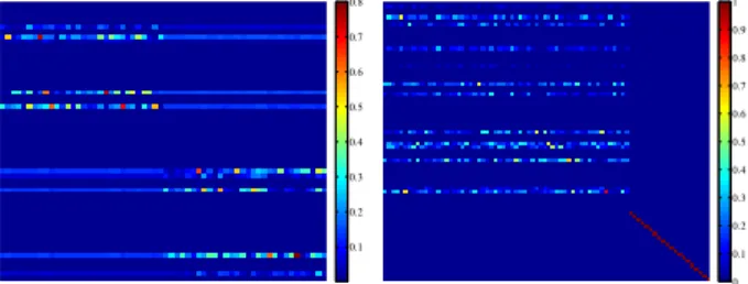
Figure 3.Left: coefficient matrix corresponding to data from two sub-spaces. Right: coefficient matrix corresponding to a dataset contaminated with outliers. The last set of points corresponds to outliers.
The optimization program (14) can also address the connectivity issues [32] of subspace clustering algorithms based on sparse representation [11,15,35] or low-rank rep-resentation [18,29]. More precisely, as discussed in [15], adding a regularizer of the formkCk1,2 to the sparse [11] or low-rank [29] objective function improves the connectiv-ity of the points in each subspace, preventing the points in a subspace to be divided into multiple components of the similarity graph.
5. Practical Considerations and Extensions
We now discuss some of the practical problems related to finding representative points of real datasets.5.1. Dealing with Outliers
In many real-world problems, the collection of data in-cludes outliers. For example, a dataset of natural scenes, objects, or faces collected from the internet can contain im-ages that do not belong to the target category. A method that robustly finds true representatives for the dataset is of par-ticular importance, as it reduces the redundancy of the data and removes points that do not really belong to the dataset. In this section, we discuss how our method can directly deal with outliers and robustly find representatives for datasets.
We use the fact that outliers are often incoherent with respect to the collection of the true data. Hence, an out-lier prefers to write itself as an affine combination of itself, while true data points choose points among themselves as representatives as they are more coherent with each other. In other words, if we denote the inliers byY and the out-liers byYo∈Rm×No, for the optimization program
minkCk1,q
s.t.
Y Yo=Y YoC, 1>C =1>,
(15)
we expect the solution to have the structure
C∗=
∆ 0
0 INo
. (16)
In other words, each outlier is a representative of itself, as shown in the right plot of Figure 3. We can therefore
identify the outliers by analyzing the row-sparsity of the solution. Among the rows of the coefficient matrix that correspond to the representatives, the ones that have many nonzero elements correspond to the true data, and the ones that have just one nonzero element correspond to outliers.
In practice,C∗might not have exactly the form of (16). However, we still expect that an outlier take part in the rep-resentation of only a few other outliers or true data points. Hence, the rows of C∗ corresponding to outliers should have very few nonzero entries. To detect and reject outliers, we define therow-sparsity index of each candidate repre-sentative`as
rsi(`) = N
c`
∞−
c`
1
(N−1)kc`k
1
∈[0,1].4 (17) For a row corresponding to an outlier, which has one or a few nonzero elements, the rsi value is close to1, while for a row which corresponds to a true representative the rsi is close to zero. Hence, we can reject outliers by selecting representatives whose rsi value is larger than a thresholdδ.
5.2. Dealing with New Observations
An important problem in finding representatives is to update the set of representative points when new data are added to the dataset. LetY be the collection of points that has already been in the dataset andYnewbe the new points
that are added to the dataset. In order to find the represen-tatives for the whole dataset including the old and the new data, one has to solve the optimization program
minkCk1,q
s.t. Y Ynew
=Y Ynew
C, 1>C=1>. (18)
However, note that we have already found the representa-tives ofY, denoted byYrep, which can efficiently describe
the collection of data inY. Thus, it is sufficient to see if the elements ofYrep are a good representative of the new
data Ynew, or equivalently, update the representatives so
that they can well describe the elements ofYrepas well as Ynew. Thus, we can solve the optimization program
minkCk1,q
s.t. Yrep Ynew
=Yrep Ynew
C, 1>C=1>, (19)
on the reduced dataset
Yrep Ynew
, which is typically of much smaller size thanY Ynew
, hence it can be solved more efficiently.5
Using similar ideas we can also deal with large datasets using a hierarchical framework. More specifically, we can
4We use the fact that forc∈
RNwe havekck1/N≤ kck∞≤ kck1.
5In general, we can minimizekQCk
1,q, for a diagonal nonnegative matrixQ, which gives relative weights to keeping the old representatives and selecting new representatives.
Event 1 Event 2 Event 3 Event 4 Event 5 Event 6 0
1 2 3 4 5 6
Number of Representatives
Tennis Match Video
λ = λ 0 / 2 λ = λ
0 / 5 λ = λ
0 / 10
Event 1 Event 2 Event 3 Event 4 Event 5 Event 6 Event 7 0
1 2 3 4 5 6
Number of Representatives
Political Debate Video λ = λ
0 / 2 λ = λ
0 / 5 λ = λ
0 / 10
Figure 4.Number of representatives for each event in the video found by our method for several values of the regularization parameter. Left: Tennis match video. Right: Political debate video.
divideY intoY1, . . . ,Y`, and find the representatives for each portion of the data, i.e., Yrep,1, . . . ,Yrep,`. Finally, we can obtain the representatives by solving the proposed optimization programs for
Yrep,1 . . . Yrep,`.
6. Experimental Results
In this section, we evaluate the performance of the pro-posed algorithm for finding representatives of real datasets on several illustrative problems. Since, using Lagrange multipliers, either of the proposed optimization programs in (7) or (10) can be written as
minλkCk1,q+1
2kY −Y Ck
2 F s.t. 1
>C =1>, (20) in practice, we use (20) for finding the representatives. We implement the algorithm using an Alternating Direction Method of Multipliers (ADMM) optimization framework [20]. As data points with very small pairwise coherences may lead to too-close representatives, similar to sparse dic-tionary learning methods [1], one can prune the set of rep-resentatives from having too-close data points.
6.1. Video Summarization
We first demonstrate the applicability of our proposed algorithm for summarizing videos. First, we consider a
1,536-frame video taken from [39], which consists of a se-ries of continuous activities with a fixed background (a few frames are shown in Figure1). We apply our algorithm in (20) and obtain 9 representatives for the whole video. The representatives are shown as frames inside the red rectan-gles. A summary of the video is provided in the caption of Figure1. Note that the representatives obtained by our al-gorithm captured the main events of the video. Perhaps the only missing representative to have a complete description of the whole video is the frame where the man is passing the tiara to the bandit (second row).
Next, we consider a video sequence of a Tennis match (a few frames are shown in Figure 2). The video consists of multiple shots of different scenes where each shot con-sists of a series of activities. We apply our algorithm in (20) and obtain11representatives for the whole video, which are shown in Figure2as frames inside the red rectangles. For
Figure 5.Representatives found by our algorithm for the images of digit
2. Note that the representatives capture different variations of the digit.
the first and the last shots, which consist of more activities relative to the other shots, we obtain 4 and3 representa-tive frames, respecrepresenta-tively. On the other hand, for the middle shots, which are shorter and have less activities, we obtain a single representative frame.
To investigate the effect of changing the regularization parameterλin the quality of obtaining representatives, we consider the tennis match video as well as a political de-bate video. We run our proposed algorithm withλ=λ0/α, whereα >1andλ0is analytically computed from the data [10]. Figure4shows the number of representatives found by our method for each of the events in the videos for sev-eral values ofα. Note that first, we always obtain one or several representatives for each of the events. Second, in both videos, the number of representatives for each event does not change much as we change the regularization pa-rameter. Finally, depending on the amount of activities in an event, we obtain an appropriate number of representa-tives for that event.
6.2. Classification Using Representatives
We now evaluate the performance of our method as well as other algorithms for finding representatives that are used for classification. For training data in each class of a dataset, we find the representatives and use them as a reduced train-ing dataset to perform classification. Ideally, if the represen-tatives are informative enough about the original data, the classification performance using the representatives should be close to the performance using all the training data. Therefore, representatives not only summarize a dataset and reduce the data storage requirements, but also can be effec-tively used for tasks such as classification and clustering.
We compare our proposed algorithm, which we call as Sparse Modeling Representative Selection (SMRS), with several standard methods for finding representatives of datasets: Kmedoids, Rank Revealing QR (RRQR) and sim-ple random selection of training data (Rand). We evaluate the classification performance using several standard clas-sification algorithms: Nearest Neighbor (NN) [9], Nearest Subspace (NS) [22], Sparse Representation-based Classi-fication (SRC) [40], and Linear Support Vector Machine (SVM) [9]. The experiments are run on the USPS dig-its database [23] and the Extended YaleB face database [28].6 For each class, we randomly select1,000 (USPS) 6USPS digits database consists of10classes corresponding to hand-written digits0,1, . . . ,9. Extended YaleB face database consists of38
Table 1.Classification Results on the USPS digit database using25 rep-resentatives of the1,000training samples in each class.
NN NS SRC SVM Rand 76.4% 84.9% 83.5% 98.6%
Kmedoids 86.0% 89.7% 89.6% 99.2%
RRQR 59.1% 81.3% 78.3% 94.3%
SMRS 83.4% 93.8% 91.7% 99.7%
All Data 96.2% 96.4% 98.9% 99.7%
Table 2.Classification Results on the Extended YaleB face database using
7representatives of the51training samples in each class. NN NS SRC SVM Rand 30.4% 71.3% 82.6% 87.9%
Kmedoids 37.9% 80.0% 89.1% 94.5%
RRQR 32.2% 88.3% 92.9% 95.3%
SMRS 33.8% 84.0% 93.1% 96.8%
All Data 72.6% 96.0% 98.2% 99.4%
/51(YaleB) of the samples for training and obtain the rep-resentatives and use the remaining samples in each class for testing. We apply our algorithm in (20) with a fixedλfor all classes, which selects, on average,25representatives for each class of the USPS database (Figure5) and7 represen-tatives for each class of the Extended YaleB database. To have a fair comparison, we select the same number of rep-resentatives using Rand, Kmedoids7, and RRQR. We also compute the classification performance using all the train-ing data. Tables 1 and2 show the results for the USPS database and the Extended YaleB database, respectively. From the results, we make the following conclusions:
a– SVM, SRC and NS work well with the representatives found by our method. Note that SRC works well when the data in each class lie in a union of low-dimensional subspaces [12,14], and, NS works well when the data in each class lie in a low-dimensional subspace. On the other hand, as we discussed earlier, our algorithm can deal with data lying in a union of subspaces, finding representatives from each subspace, justifying its compatibility with both SRC and NS. The good performance of the NS in Table2
using the representatives obtained by RRQR comes from the fact that the data in each class of the Extended YaleB dataset can be well modeled by a single low-dimensional subspace [3,28], which is the underlying assumption be-hind the RRQR algorithm for finding the representatives.
b– For the NN method to work well, we often need to have enough samples from each class so that given a test sam-ple, its nearest neighbor comes from the right class. Thus, methods such as Kmedoids that look for the centers of the data distribution in each class perform better with NN. For classes of face images corresponding to different individuals captured un-der a fixed pose and varying illumination.
7Since Kmedoids depends on initialization, we use100restarts of the algorithm and take the result that obtains the minimum energy.
10% 20% 30% 40% 50% 0
0.1 0.2 0.3 0.4 0.5 0.6 0.7 0.8 0.9
Percentage of Outliers
Percentage of Outlier Representatives
Kmedoids RRQR SMRS SMRS−rsi
0 0.2 0.4 0.6 0.8 1 0
0.1 0.2 0.3 0.4 0.5 0.6 0.7 0.8 0.9 1
False Positive Rate
True Positive Rate
ROC Curves
10% outliers 20% outliers 30% outliers 40% outliers 50% outliers
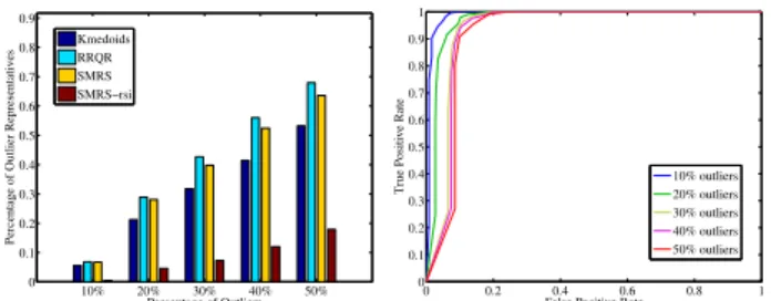
Figure 6.Left: percentage of outlier representatives for different algo-rithms as a function of the percentage of outliers in the dataset. Right: ROC curves for the proposed method for different percentages of outliers. the NN method in the Extended YaleB dataset, the large gap between using all the training data and using the rep-resentatives obtained by different algorithms is mainly due the fact that the data in different classes are close to each other [13,15], hence using a subset of the the training data can significantly change the inter and intra class distances of the training data.
6.3. Outlier Rejection
To evaluate the performance of our algorithm for reject-ing outliers, we form a dataset ofN = 1,024images, where
(1−ρ)fraction of the images are randomly selected from the Extended YaleB face database. The remaining ρ frac-tion of the data, which correspond to outliers, are random images downloaded from the internet. For different values ofρin{0.1,0.2,0.3,0.4,0.5}, we run our algorithm as well as Kmedoids and RRQR to select roughly100 representa-tives for the dataset. Figure6(left) shows the percentage of outliers among the representatives as we increase the num-ber of outliers in the dataset. We show the result of our algorithm prior to and after rejecting representatives using rsi > δ, where for all values of ρwe setδ = 0.16. As expected, the percentage of outliers among representatives increases as the number of outliers in the dataset increases. Also, all methods, select roughly the same number of out-liers in their representatives. However, note that our pro-posed algorithm has the advantage of detecting and reject-ing outliers by simply analyzreject-ing the row-sparsity of the co-efficient matrixC. As shown in the plot, by removing the representatives whose rsi value is greater thanδ= 0.16, the number of outlier representatives significantly drops for our algorithm (we still keep at least90% of the true represen-tatives as shown in the ROC curves). Figure6also shows the ROC curves of our method for different percentages of outliers in the dataset. Note that, for all values of ρ, we can always obtain a high positive rate,i.e., keep many true representatives, with a relatively low false positive rate,i.e., select very few outliers in the representatives.
7. Discussion
We proposed an algorithm for finding a subset of the data points in a dataset as the representatives. We assumed that
each data point can be expressed efficiently as a combina-tion of the representatives. We cast the problem as a joint sparse multiple measurement vector problem where both the dictionary and the measurements are given by the data points and the unknown sparse codes select the represen-tatives. For a convex relaxation of the original nonconvex formulation, we showed the relationship of the representa-tives to the vertices of the convex hull of the data. It is important to note that the convex relaxation takes into ac-count the value of the norm of the coefficients, hence prefers representatives with such geometrical properties. As we show in [10], greedy algorithms that are insensitive to the norm of the coefficients lead to representatives with differ-ent geometrical properties. When the data come from a col-lection of low-rank models, under appropriate conditions, we showed that our proposed algorithm selects represen-tatives from each low-rank model. It is important to note that our proposed algorithm also allows to incorporate the prior knowledge about the nonlinear structure of the data using kernel methods and weighting the coefficient matrix into the optimization program [10].
Acknowledgment
E. Elhamifar would like to thank Ewout van den Berg for fruit-ful discussions about the paper. E. Elhamifar and R. Vidal are sup-ported by grants NSF CNS-0931805, NSF ECCS-0941463, NSF OIA-0941362, and ONR N00014-09-10839. G. Sapiro acknowl-edges the support by DARPA, NSF, and ONR grants.
References
[1] M. Aharon, M. Elad, and A. M. Bruckstein. The k-svd: An algorithm for designing of overcomplete dictionaries for sparse representations. IEEE TIP, 2006.2,3,6
[2] L. Balzano, R. Nowak, and W. Bajwa. Column subset selection with missing data.NIPS Workshop on Low-Rank Methods for Large-Scale Machine Learning, 2010.1
[3] R. Basri and D. Jacobs. Lambertian reflection and linear subspaces. IEEE TPAMI, 2003.7
[4] S. Bengio, F. Pereira, Y. Singer, and D. Strelow. Group sparse coding. NIPS, 2009.2
[5] C. Boutsidis, M. W. Mahoney, and P. Drineas. An improved approxi-mation algorithm for the column subset selection problem. Proceed-ings of SODA, 2009.1
[6] T. Chan. Rank revealing qr factorizations. Lin. Alg. and its Appl., 1987.1
[7] R. Coifman and S. Lafon. Diffusion maps. Applied and Computa-tional Harmonic Analysis, 2006.1
[8] D. L. Donoho. Neighborly polytopes and sparse solution of under-determined linear equations.(preprint), 2004.4
[9] R. Duda, P. Hart, and D. Stork. Pattern Classification. Wiley-Interscience, 2004.6
[10] E. Elhamifar, G. Sapiro, and R. Vidal. Sparse modeling for finding representative objects.in preparation.4,6,8
[11] E. Elhamifar and R. Vidal. Sparse subspace clustering.CVPR, 2009. 2,5
[12] E. Elhamifar and R. Vidal. Robust classification using structured sparse representation.CVPR, 2011.7
[13] E. Elhamifar and R. Vidal. Sparse manifold clustering and embed-ding.NIPS, 2011.7
[14] E. Elhamifar and R. Vidal. Block-sparse recovery via convex opti-mization.IEEE TSP, 2012.7
[15] E. Elhamifar and R. Vidal. Sparse subspace clustering: Algo-rithm, theory, and applications.IEEE TPAMI, submitted., Available: http://arxiv.org/abs/1203.1005.2,5,7
[16] K. Engan, S. O. Aase, and J. H. Husoy. Method of optimal directions for frame design.ICASSP, 1999.3
[17] E. Esser, M. Moller, S. Osher, G. Sapiro, and J. Xin. A con-vex model for non-negative matrix factorization and dimension-ality reduction on physical space. Technical report, Available: http://arxiv.org/abs/1102.0844, 2011.1,2
[18] P. Favaro, R. Vidal, and A. Ravichandran. A closed form solution to robust subspace estimation and clustering.CVPR, 2011.2,5 [19] B. J. Frey and D. Dueck. Clustering by passing messages between
data points.Science, 2007.1
[20] D. Gabay and B. Mercier. A dual algorithm for the solution of non-linear variational problems via finite-element approximations.Comp. Math. Appl., 1976.6
[21] M. Gu and S. C. Eisenstat. Efficient algorithms for computing a strong rank-revealing qr factorization. SIAM Journal on Scientific Computing, 1996.1
[22] J. Ho, M. H. Yang, J. Lim, K. Lee, and D. Kriegman. Clustering appearances of objects under varying illumination conditions.CVPR, 2003.6
[23] J. J. Hull. A database for handwritten text recognition research.IEEE TPAMI, 1994.6
[24] R. Jenatton, J. Y. Audibert, and F. Bach. Structured variable selection with sparsity-inducing norms.JMLR, 2011.2
[25] I. Jolliffe.Principal Component Analysis. Springer, 2002.1,3 [26] L. Kaufman and P. Rousseeuw. Clustering by means of medoids.
In Y. Dodge (Ed.), Statistical Data Analysis based on the L1 Norm (North-Holland, Amsterdam), 1987.1
[27] N. Keshava and J. Mustard. Spectral unmixing. IEEE Signal Pro-cessing Magazine, 2002.1
[28] K. C. Lee, J. Ho, and D. Kriegman. Acquiring linear subspaces for face recognition under variable lighting.IEEE TPAMI, 2005.6,7 [29] G. Liu, Z. Lin, and Y. Yu. Robust subspace segmentation by low-rank
representation.ICML, 2010.2,5
[30] J. Mairal, F. Bach, J. Ponce, G. Sapiro, and A. Zisserman. Discrimi-native learned dictionaries for local image analysis.CVPR, 2008.2, 3
[31] J. Mairal, F. Bach, J. Ponce, G. Sapiro, and A. Zisserman. Non-local sparse models for image restoration.ICCV, 2009.2,3
[32] B. Nasihatkon and R. Hartley. Graph connectivity in sparse subspace clustering. InCVPR, 2011.5
[33] I. Ramirez, P. Sprechmann, and G. Sapiro. Classification and clus-tering via dictionary learning with structured incoherence and shared features.CVPR, 2010.2,3
[34] S. Roweis and L. Saul. Nonlinear dimensionality reduction by locally linear embedding.Science, 2000.1
[35] M. Soltanolkotabi and E. J. Candes. A geometric anal-ysis of subspace clustering with outliers. Available: http://arxiv.org/abs/1112.4258.5
[36] J. B. Tenenbaum, V. de Silva, and J. C. Langford. A global geometric framework for nonlinear dimensionality reduction.Science, 2000.1 [37] J. A. Tropp. Algorithms for simultaneous sparse approximation. part ii: Convex relaxation. Signal Processing, special issue ”Sparse ap-proximations in signal and image processing”, 2006.2
[38] J. A. Tropp. Column subset selection, matrix factorization, and eigenvalue optimization.Proceedings of SODA, 2009.1
[39] R. Vidal. Recursive identification of switched ARX systems. Auto-matica, 2008.6
[40] J. Wright, A. Yang, A. Ganesh, S. Sastry, and Y. Ma. Robust face recognition via sparse representation.IEEE TPAMI, 2009.6