Enhancing the Solution Method of Linear Tri-Level
Programming Problem Utilizing a New heuristic
approach
Eghbal Hosseini
Ph.D. Candidate
Department of Mathematics,
Payamenur University of Tehran,
Iran.
Isa Nakhai Kamalabadi
Professor
Industrial Engineering at
University of Kurdistan,Sanandaj,
Iran.
ABSTRACT
In the recent years, the bi-level and tri-level programming problems (TLPP) are interested by many researchers and TLPP is known as an appropriate tool to solve the real problems in several areas such as economic, traffic, finance, management, and so on. Also, it has been proven that the general TLPP is an NP-hard problem. The literature shows a few attempts for using exact methods. In this paper, we attempt to develop an effective approach based on analyze theorems for solving the linear TLPP. In this approach, by using the heuristic method the TLPP is converted to a linear single problem. Finally, the single level problem is solved using the enumeration algorithm. The presented approach achieves an efficient and feasible solution in an appropriate time which has been evaluated by comparing to references and test problems.
Keywords:
Linear bi-level programming problem, linear tri -level programming problem, heuristic method, enumeration algorithm.1.
INTRODUCTION
It has been proved that the BLP is NP- Hard problem even to seek for the locally optimal solutions (Bard, 1991; Vicente, et al., 1994)[3, 23]. Nonetheless the BLPP is an applicable problem and practical tool to solve decision making problems. It is used in several areas such as transportation, finance and so on. Therefore finding the optimal solution has a special importance to researchers.
Several algorithms have been presented for solving the BLP (Yibing, et al., 2007; Allende & G. Still,
approaches (Hejazi, et al., 2002; Wang et al., 2008; Hu, et al., 2010; Baran Pal, et al., 2010; Wan et al., 2012; Yan, et al., 2013; Kuen-Ming et al., 2007, Hosseini, E and I.Nakhai Kamalabadi., 2013, He, X and C. Li, T. Huang, 2014) [11, 25, 12, 4, 26, 29, 14, 8, 9, 7].
However several algorithms have been proposed to BLPP, a few algorithms have been proposed to solve TLPP (Zhang , et al., 2010) [31].
The remainder of the paper is structured as follows: in Section 2, basic concepts of the linear BLPP and TLPP are introduced. We provide the proposed heuristic algorithm for solving the TLPP in Section 3. Computational results are presented for our approach in Section 4. Finally, the paper is finished in Section 5 by presenting the concluding remarks.
2.
The linear bi-level and tri-level programming problems
In this section models of bi-level and tri-level programming problems are introduced.
BLPP is used frequently by problems with decentralized planning structure. It is defined as [20]:
min
x F x, y = a
Tx + bTy
s. t min
y g x, y = c
Tx + dTy
Ax + By ≤ r,
x, y ≥ 0.
(1)
where a, c ∈ Rn1. b, d ∈ Rn2, A ∈ Rm×n1. B ∈ Rm×n2, r ∈ Rm, x ∈ Rn1, y ∈ Rn2 and 𝐹(𝑥, 𝑦) and 𝑔(𝑥, 𝑦) are the objective
functions of the leader and the follower, respectively.
In general, BLPP is a non-convex optimization problem; therefore, there is no general algorithm to solve it. This problem can be non-convex even when all functions and constraints are bounded and continuous. Of course, the linear BLPP is convex and preserving this property is very important. A summary of important properties for convex problem are as follows, which 𝐹: 𝑆 𝑅. 𝑛 and 𝑆 is a nonempty convex set in 𝑅𝑛:
(1) The convex function f is continuous on the interior of 𝑆.
(2) Every local optimal solution of 𝐹 over a convex set 𝑋 ⊆ 𝑆 is the unique global optimal solution. (3) If 𝛻𝐹 𝑥 = 0, then 𝑥 is the unique global optimal solution of 𝐹 over 𝑆.
Because a tri-level decision reflects the principle features of multi-level programming problems, the algorithms developed for tri-level decisions can be easily extended to multi-level programming problems which the number of levels is more than three. Hence, just tri-level programming is studied in this paper.
min
x 𝐹1 x, y, z = 𝑎1x + 𝑏1y + 𝑐1𝑧
𝐴1x + 𝐵1y + 𝐶1z ≤ 𝑟1,
s. t min
y 𝐹2 x, y, z = 𝑎2x + 𝑏2y + 𝑐2𝑧
𝐴2x + 𝐵2y + 𝐶2z ≤ 𝑟2,
s. t min
z 𝐹3 x, y, z = 𝑎3x + 𝑏3y + 𝑐3𝑧
𝐴3x + 𝐵3y + 𝐶3z ≤ 𝑟3,
x, y, z ≥ 0.
(2)
Where 𝐴𝑖 ∈ Rq×k, 𝐵𝑖 ∈ Rq×l, 𝐶𝑖 ∈ Rq×p, 𝑟𝑖 ∈ Rq, x ∈ Rk, y ∈ Rl, z ∈ Rp, 𝑎𝑖∈ Rk, 𝑏𝑖 ∈ Rl, 𝑐𝑖 ∈ R𝑝, i = 1,2,3, and the variables x, y, z are called the top-level, middle-level, and bottom-level variables respectively,
𝐹1 x, y, z , 𝐹2 x, y, z , 𝐹3 x, y, z , the top-level, middle-level, and bottom-level objective functions, respectively. In this problem each level has individual control variables, but also takes account of other levels’ variables in its optimization function.
To obtain an optimized solution to TLP problem based on the solution concept of bi-level programming [6], we first introduce some definitions and notation:
Definition 2.1
The feasible region of the TLP problem when i=1,2,3, is
S = (x, y, z) 𝐴𝑖x + 𝐵𝑖y + 𝐶𝑖z ≤ 𝑟𝑖 , x, y, z ≥ 0. (3)
On the other hand, if x be fixed, the feasible region of the follower can be explained as
S = (y, z) 𝐵𝑖y + 𝐶𝑖z ≤ 𝑟𝑖− 𝐴𝑖x , y, z ≥ 0 . (4)
Based on the above assumptions, the follower rational reaction set is
P x = {(y, z) ∈ argming x, y, z , (y, z) ∈ S x }. (5)
Where the inducible region is as follows
IR = { x, y, z ∈ S, (y, z) ∈ P x }. (6)
Finally, the tri-level programming problem can be written as
min{F(x, y, z)|(x, y, z) ∈ IR}. (7)
S = x, y, z 𝐴𝑖x + 𝐵𝑖y + 𝐶𝑖z ≤ 𝑟𝑖, x, y, z ≥ 0 (8)
Definition 2.2:
Every point such as (x, y, z)is a feasible solution to tri-level problem if (x, y, Z) ∈ IR
Definition 2.3:
Every point such as (x∗, y∗, z∗) is an optimal solution to the tri-level problem if
F x∗. y∗, z∗ ≤ F x, y, z ⩝ x, y, z ∈ IR. (9)
3.
Heuristic algorithm (HA) to solve TLPP
A.
Main Theoretical Concepts
In this section, main concepts and essential theorems in order to expansion of our algorithm are discussed.
Definition 3.1:
If X be a bounded above set, then the least upper bound of X is called supreme and it is exhibited by Sup(X) and:
∀𝑥 ∈𝑋 𝑆𝑢𝑝 𝑋 ≥ 𝑥.
Definition 3.2:
If X be a bounded below set, then the greatest lower bound of X is called infimum and it is exhibited by Inf(X) and:
∀𝑥∈𝑋 𝐼𝑛𝑓 𝑋 ≤ 𝑥.
Theorme 3.1:
If X be a bounded aboveset and 𝑎 = 𝑆𝑢𝑝 𝑋 then for every small positive number such as ℇ:
Proof :
The proof is simple. Let 𝑎 + ℇ ∈ X.
Because ℇ is positive then 𝑎 + ℇ > 𝑎 and 𝑎 can not be supreme of X by defenition 1.
This is contradiction with supposition 𝑎 = 𝑆𝑢𝑝 𝑋 . Therfore this assumption that 𝑎 + ℇ ∈ X is false and then Hence proof of theorem finished.
Theorme 3.2:
If X be a bounded belowset and 𝑏 = 𝐼𝑛𝑓 𝑋 , then for every small positive number such as ℇ:
Proof :
Let 𝑏 − ℇ ∈ X
X a
X b
Because ℇ is positive then 𝑏 − ℇ < 𝑏 and 𝑏 can not be supreme of X by defenition 1.
This is contradiction with supposition 𝑏 = 𝐼𝑛𝑓 𝑋 . Therfore this assumption that 𝑏 − ℇ ∈ X is false and then Hence proof of theorem finished.
Theorme 3.3 [20]:
If X be a bounded and non- empty set then min 𝑋 = inf 𝑋 , max 𝑋 = sup 𝑋 . Proof :
Theproof of this theorem was given by [20].
Now consider the problem (2), in this paper we suppose X, feasible space of (2), is a bounded set.
Let
u = 𝑎2x + 𝑏2y + 𝑐2𝑧 , 𝑤 = 𝑎3x + 𝑏3y + 𝑐3𝑧 (10)
then:
z = 𝑐2−1(u − 𝑎2x − 𝑏2y) (11)
And
𝑤 = 𝑎3x + 𝑏3y + 𝑐3𝑐2−1 u − 𝑎2x − 𝑏2y (12)
Therefore
𝑦 = 𝑏3− 𝑐3𝑐2−1𝑏2 −1 𝑤 − 𝑎3x − 𝑐3𝑐2−1𝑢 + 𝑐3𝑐2−1𝑎2𝑥 (13)
Equation (11) is valid because x and y are fixed in the last level and they are controlled by the first and middle levels, therefore the last problem has only z as variable. By substituting equation (11) in (13), the problem (2) converts to the following single problem:
min.𝑎1𝑥 + 𝑏1( 𝑏3− 𝑐3𝑐2−1𝑏2 −1 𝑤 − 𝑎3x − 𝑐3𝑐2−1𝑢 + 𝑐3𝑐2−1𝑎2𝑥 ) + 𝑐1(𝑐2−1(u − 𝑎2x −
𝑏2(𝑏3−𝑐3𝑐2−1𝑏2−1𝑤−𝑎3x−𝑐3𝑐2−1𝑢+𝑐3𝑐2−1𝑎2𝑥)))
s. t 𝐴1x + 𝐵1( 𝑏3− 𝑐3𝑐2−1𝑏2 −1 𝑤 − 𝑎3x − 𝑐3𝑐2−1𝑢 + 𝑐3𝑐2−1𝑎2𝑥
+ 𝐶1(𝑐2−1 u − 𝑎2x − 𝑏2( 𝑏3− 𝑐3𝑐2−1𝑏2 −1 𝑤 − 𝑎3x − 𝑐3𝑐2−1𝑢 + 𝑐3𝑐2−1𝑎2𝑥 ) ) ≤ 𝑟1,
𝐴2x + 𝐵2( 𝑏3− 𝑐3𝑐2−1𝑏2 −1 𝑤 − 𝑎3x − 𝑐3𝑐2−1𝑢 + 𝑐3𝑐2−1𝑎2𝑥 ) + 𝐶2(𝑐2−1(u − 𝑎2x
− 𝑏2( 𝑏3− 𝑐3𝑐2−1𝑏2 −1 𝑤 − 𝑎3x − 𝑐3𝑐2−1𝑢 + 𝑐3𝑐2−1𝑎2𝑥 ))) ≤ 𝑟2,
𝐴3x + 𝐵3( 𝑏3− 𝑐3𝑐2−1𝑏2 −1 𝑤 − 𝑎3x − 𝑐3𝑐2−1𝑢 + 𝑐3𝑐2−1𝑎2𝑥 ) + 𝐶3(𝑐2−1(u − 𝑎2x
− 𝑏2( 𝑏3− 𝑐3𝑐2−1𝑏2 −1 𝑤 − 𝑎3x − 𝑐3𝑐2−1𝑢 + 𝑐3𝑐2−1𝑎2𝑥 ))) ≤ 𝑟3,
u = α, w = β, x ≥ 0.
(14)
Which α, β are the last values of u and w (minimum of w and u). It is easy to show that by removing these two constraints:
u = α, w = β,
We can obtain a relaxation to the problem (14):
.
min.𝑎1𝑥 + 𝑏1( 𝑏3− 𝑐3𝑐2−1𝑏2 −1 𝑤 − 𝑎3x − 𝑐3𝑐2−1𝑢 + 𝑐3𝑐2−1𝑎2𝑥 ) + 𝑐1(𝑐2−1(u − 𝑎2x −
𝑏2(𝑏3−𝑐3𝑐2−1𝑏2−1𝑤−𝑎3x−𝑐3𝑐2−1𝑢+𝑐3𝑐2−1𝑎2𝑥)))
s. t 𝐴1x + 𝐵1( 𝑏3− 𝑐3𝑐2−1𝑏2 −1 𝑤 − 𝑎3x − 𝑐3𝑐2−1𝑢 + 𝑐3𝑐2−1𝑎2𝑥
+ 𝐶1(𝑐2−1 u − 𝑎2x − 𝑏2( 𝑏3− 𝑐3𝑐2−1𝑏2 −1 𝑤 − 𝑎3x − 𝑐3𝑐2−1𝑢 + 𝑐3𝑐2−1𝑎2𝑥 ) ) ≤ 𝑟1,
𝐴2x + 𝐵2( 𝑏3− 𝑐3𝑐2−1𝑏2 −1 𝑤 − 𝑎3x − 𝑐3𝑐2−1𝑢 + 𝑐3𝑐2−1𝑎2𝑥 ) + 𝐶2(𝑐2−1(u − 𝑎2x
− 𝑏2( 𝑏3− 𝑐3𝑐2−1𝑏2 −1 𝑤 − 𝑎3x − 𝑐3𝑐2−1𝑢 + 𝑐3𝑐2−1𝑎2𝑥 ))) ≤ 𝑟2,
𝐴3x + 𝐵3( 𝑏3− 𝑐3𝑐2−1𝑏2 −1 𝑤 − 𝑎3x − 𝑐3𝑐2−1𝑢 + 𝑐3𝑐2−1𝑎2𝑥 ) + 𝐶3(𝑐2−1(u − 𝑎2x
− 𝑏2( 𝑏3− 𝑐3𝑐2−1𝑏2 −1 𝑤 − 𝑎3x − 𝑐3𝑐2−1𝑢 + 𝑐3𝑐2−1𝑎2𝑥 ))) ≤ 𝑟3,
x ≥ 0.
(15)
Let X and S are feasible spaces of (14), (15) respectively. The problem (15) is a single linear programming problem and the optimal solution of linear problems is a vertex point. To obtain optimal solution, problem (15) will be solved by the proposed algorithm and it calculates all the vertex points in S. We necessary vertex point in X and some of vertex points in S will be removed by theorems because u and w should be Minimum in other words u = α,w = β.
According to the theorems 1, 2, 3 it is easy to see that the following relations are contradictory with to minimize u and w:
x, u, w ∈ S & x, u − ℇ, w − ℇ ∈ S x, u, w ∈ S & x, u, w − ℇ ∈ S x, u, w ∈ S & x, u − ℇ, w ∈ S
Therefore if , then x, u, w ∈ X.
Using the proposed algorithm and theorems all the vertex points in S are obtained and the optimal solution is calculated by enumeration method.
B.
Steps of the algorithm
In this section, steps of presented algorithm are proposed.
Step 1: We suppose that theobjective function of the follower be a new variable and replace it in the leader objective function. Therefore the BLPP is changed into a single level problem. By applying this step, problem (9) is converted into (12) which are in linear form.
Step 2: The constraints related to u and w, two new variables which equal to the middle and the last objective functions, are removed to obtain problem (14) (a relaxation to (15)).
Step 3: Finding all vertex points in problem (15). A vertex point is found by solving at least two constraints for a problem which has two variables. Also solving three constraints give a vertex point for a problem which has three variables and so on. These vertex points can be infeasible in (14). Step 4 proposes all feasible vertex points to problem (14).
Step 4: According to the proposed theorems each vertex point such as (𝑥, 𝑢, 𝑤) in S (feasible space of the problem (15) is a vertex point to X (feasible space of the problem (14)) if only if for each small positive number ℇ:
When the follower problem is minimization and
S w
u
x, , )
(
S w
u
x, , )
(
S w
u
x, , )
When the follower problem is maximization . To minimization:
To maximization:
Objective functions correspond feasible vertex points in (11) are recorded.
Step 5: Finding the best objective function among recorded objective functions in step 4 as the best solution to BLPP.
4.
Computational results
To illustrate the algorithm, we consider the following examples.
Example 1 [38]:
Consider the following linear tri-level programming problem:
min
x x − 4y + 2z
s. t
−x − y ≤ −3, −3 x + 2y − z ≥ −10, min
y 𝑥 + 𝑦 − 𝑧 s. t
−2 x + y − 2z ≤ −1, 2x + y + 4z ≤ 14, min
y 𝑥 − 2𝑦 − 2𝑧
s. t
2x − y − z ≤ 2, x, y, z ≥ 0.
Using (10-12) let
u = 𝑥 + 𝑦 − 𝑧 , 𝑤 = 𝑥 − 2𝑦 − 2𝑧
Then:
z = −u + x + y
And
w = 𝑥 − 2𝑦 − 2(−𝑢 + 𝑥 + 𝑦)
Therefore
𝑦 = −1
4 𝑤 + x − 2𝑢
the above problem is changed to the following problem:
) 16 ( X w u x S w u x S w u
x, , ) ,( , , ) ( , , )
(
X w u x S w u x S w ux, , ) ,( , , ) ( , , )
min
x x − 4(−
1
4 𝑤 + x − 2𝑢 ) + 2(−u + x + y)
s. t
−x − (−1
4 𝑤 + x − 2𝑢 ) ≤ −3,
−3 x + 2(−1
4 𝑤 + x − 2𝑢 ) − (−u + x + y) ≥ −10,
−2 x + (−1
4 𝑤 + x − 2𝑢 ) − 2(−u + x + y) ≤ −1,
2x + (−1
4 𝑤 + x − 2𝑢 ) + 4(−u + x + y) ≤ 14,
2x − (−1
4 𝑤 + x − 2𝑢 ) − (−u + x + y) ≤ 2, x ≥ 0,
u = α, w = β.
Which α , β are the smallest values of u, w. The two last constraints are removed and the following relaxation is obtained:
min x − 4(−1
4 𝑤 + x − 2𝑢 ) + 2(−u + x + − 1
4 𝑤 + x − 2𝑢 )
s. t
−x − (−1
4 𝑤 + x − 2𝑢 ) ≤ −3,
−3 x + 2(−1
4 𝑤 + x − 2𝑢 ) − (−u + x + − 1
4 𝑤 + x − 2𝑢 ) ≥ −10,
−2 x + (−1
4 𝑤 + x − 2𝑢 ) − 2(−u + x + − 1
4 𝑤 + x − 2𝑢 ) ≤ −1,
2x + (−1
4 𝑤 + x − 2𝑢 ) + 4(−u + x + − 1
4 𝑤 + x − 2𝑢 ) ≤ 14,
2x − (−1
4 𝑤 + x − 2𝑢 ) − (−u + x + − 1
4 𝑤 + x − 2𝑢 ) ≤ 2, x ≥ 0.
Using enumeration method some of the vertex points are:
4,10, −8 , 0, −2,4 , 3,0, −4 , −1.5, −5.8, −4.7 , 1,2.25,3.6 , 0,0,0 , 5,0,4 , 1,1, −7 , 1,2, −3 , 2,6, −10 , …
Now we have:
0, −2 − 𝜀, 4 − 𝜀 ∈ 𝑆, 3,0 − 𝜀, −4 − 𝜀 ∈ 𝑆, −1.5, −5.8 − 𝜀, −4.7 − 𝜀 ∈ 𝑆, 1,2.25 − 𝜀, 3.6 − 𝜀 ∈ 𝑆
According to the Step 4, all the recent vertex points are infeasible and:
4,10 − 𝜀, −8 − 𝜀 , 1,1 − 𝜀, −7 − 𝜀
1,2 − 𝜀, −3 − 𝜀 , 2,6 − 𝜀, −10 − 𝜀
S
S
S
Therefore the problem has just this feasible vertex points:
4,10, −8 , 1,1, −7 , 1,2, −3 , 2,6, −10 Table 1 – The feasible vertex points in example1
(𝑥, 𝑢, 𝑤) (𝑥, 𝑦, 𝑧) 𝐹1(𝑥, 𝑦, 𝑧)
4,10, −8 4,6,0 -20
1,1, −7 1,2,2 -3
1,2, −3 1,2,1 -5
2,6, −10 2,5,1 -16
Using above Table the optimal solution by the proposed algorithm as follows:
𝑥∗, 𝑦∗, 𝑧∗ = 4,6,0
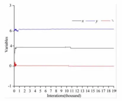
Optimal solution is presented according to Table 2. Behavior of the variables in Example 1 has been show in figure 1.
Table 2- Comparison of optimal solutions by Heuristic algorithm – Example 1.
Optimal Solution
Best solution by HA Best solution according to reference [31]
(𝑥∗, 𝑦∗, 𝑧∗) (4,6,0) (4,6,0)
𝐹1 x, y, z -20 -20
𝐹2 x, y, z 10 10
𝐹3 x, y, z -8 -8
Example 2 [38]:
Consider the following linear tri-level programming problem.
min
x x + 4y + 2z
s. t
x − 3y + 9z ≤ 30, −3 x + 5y − z ≤ −100, min
y −𝑥 + 7𝑦 − 𝑧 s. t
3x + 5y − z ≤ 160, min
y 7𝑥 + 𝑦 + 21𝑧
s. t
3x − 4y − 2z ≤ 212, x, y, z ≥ 0.
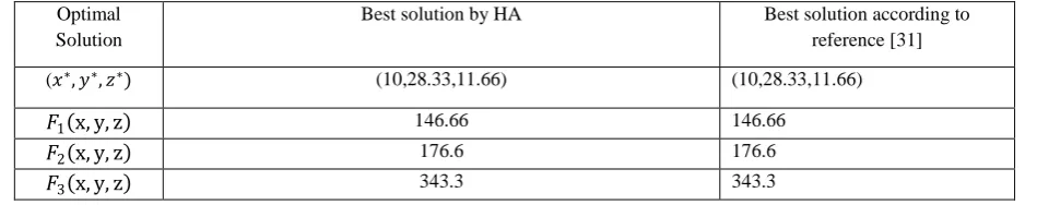
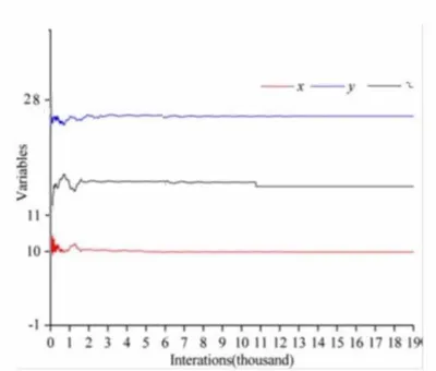
Optimal solution for this example is presented according to Table 3. Behavior of the variables has been show in figure 2.
Table 3- Comparison of optimal solutions by Heuristic algorithm – Example 2.
Optimal Solution
Best solution by HA Best solution according to reference [31]
(𝑥∗, 𝑦∗, 𝑧∗) (10,28.33,11.66) (10,28.33,11.66)
𝐹1 x, y, z 146.66 146.66
𝐹2 x, y, z 176.6 176.6
Figure 2 - Behavior of the variablesin Example 2
5.
Conclusion and future work
In this paper, we used a new heuristic approach to convert the tri level problem into a single level problem. Then, using the enumeration method all the vertex point of the linear single problem was been obtained. Utilizing the proposed mathematics analyze theorems the optimal solution was proposed. Comparing with the results of previous methods, our algorithm has better numerical results and present better solutions. The best solutions produced by proposed algorithm are exact unlike the previous best solutions by other researchers.
In the future works, the following should be researched:
(1) Examples in larger sizes can be supplied to illustrate the efficiency of the proposed algorithms.
6.
REFERENCES
[1] Allende, G and B. G. Still, Solving bi-level programs with the KKT-approach, Springer and Mathematical Programming Society (2012) 1 31:37 – 48.
[2] Arora, S.R and R. Gupta, Interactive fuzzy goal programming approach for bi-level programming problem, European Journal of Operational Research (2007) 176 1151–1166.
[3] Bard, J.F, Some properties of the bi-level linear programming, Journal of Optimization Theory and Applications (1991) 68 371–378.
[4] Bard, J.F and Practical bi-level optimization: Algorithms and applications, Kluwer Academic Publishers, Dordrecht, 1998.
[5] Dempe, S and A.B. Zemkoho, On the Karush–Kuhn–Tucker reformulation of the bi-level optimization problem, Nonlinear Analysis 75 (2012) 1202–1218.
[6] Facchinei, F and H. Jiang, L. Qi, A smoothing method for mathematical programming with equilibrium constraints, Mathematical Programming 85 (1999) 107-134.
[7] He, X and C. Li, T. Huang, C. Li, Neural network for solving convex quadratic bilevel programming problems, Neural Networks, Volume 51, March 2014, Pages 17-25.
[8] Hosseini, E and I.Nakhai Kamalabadi, A Genetic Approach for Solving Bi-Level Programming Problems, Advanced Modeling and Optimization, Volume 15, Number 3, 2013.
[9] Hosseini, E and I.Nakhai Kamalabadi, Solving Linear-Quadratic Bi-Level Programming and Linear-Fractional Bi-Level Programming Problems Using Genetic Based Algorithm, Applied Mathematics and Computational Intellegenc, Volume 2, 2013.
[10]Hosseini, E and I.Nakhai Kamalabadi, Taylor Approach for Solving Non-Linear Bi-level Programming [11]Problem ACSIJ Advances in Computer Science: an International Journal, Vol. 3, Issue 5, No.11 , September
2014.
[12]Hejazi, S.R and A. Memariani, G. Jahanshahloo, (2002) Linear bi-level programming solution by genetic algorithm, Computers & Operations Research 29 1913–1925.
[13]Hu, T. X and Guo, X. Fu, Y. Lv, (2010) A neural network approach for solving linear bi-level programming problem, Knowledge-Based Systems 23 239–242.
[14]Khayyal, A.AL Minimizing a Quasi-concave Function Over a Convex Set: A Case Solvable by Lagrangian Duality, proceedings, I.E.E.E. International Conference on Systems, Man,and Cybemeties, Tucson AZ (1985) 661-663.
[15]Kuen-Ming, L and Ue-Pyng.W, Hsu-Shih.S, A hybrid neural network approach to bi-level programming problems, Applied Mathematics Letters 20 (2007) 880–884
[16]Luce, B and Saïd.H, Raïd.M, One-level reformulation of the bi-level Knapsack problem using dynamic programming, Discrete Optimization 10 (2013) 1–10.
[17]Masatoshi, S and Takeshi.M, Stackelberg solutions for random fuzzy two-level linear programming through possibility-based probability model, Expert Systems with Applications 39 (2012) 10898–10903.
[18]Mathieu, R. and L. Pittard, G. Anandalingam, Genetic algorithm based approach to bi-level Linear Programming, Operations Research (1994) 28 1–21.
[19]Nocedal, J and S.J. Wright, 2005 Numerical Optimization, Springer-Verlag, , New York.
[20]Pramanik, S and T.K. Ro, Fuzzy goal programming approach to multilevel programming problems, European Journal of Operational Research (2009) 194 368–376.
[21]Sakava, M. and I. Nishizaki, Y. Uemura, Interactive fuzzy programming for multilevel linear programming problem, Computers & Mathematics with Applications (1997) 36 71–86.
[23]Thoai, N. V and Y. Yamamoto, A. Yoshise, (2002) Global optimization method for solving mathematical programs with linear complementary constraints, Institute of Policy and Planning Sciences, University of Tsukuba, Japan 978.
[24]Vicente, L and G. Savard, J. Judice, Descent approaches for quadratic bi-level programming, Journal of Optimization Theory and Applications (1994) 81 379–399.
[25]Wend, W. T and U. P. Wen, (2000) A primal-dual interior point algorithm for solving bi-level programming problems, Asia-Pacific J. of Operational Research, 17.
[26]Wang, G. Z and Wan, X. Wang, Y.Lv, Genetic algorithm based on simplex method for solving Linear-quadratic bi-level programming problem, Computers and Mathematics with Applications (2008) 56 2550–2555.
[27]Wan, Z. G and Wang, B. Sun, ( 2012) A hybrid intelligent algorithm by combining particle Swarm optimization with chaos searching technique for solving nonlinear bi-level programming Problems, Swarm and Evolutionary Computation.
[28]Wan, Z and L. Mao, G. Wang, Estimation of distribution algorithm for a class of nonlinear bilevel programming problems, Information Sciences, Volume 256, 20 January 2014, Pages 184-196.
[29]Xu, P and L. Wang, An exact algorithm for the bilevel mixed integer linear programming problem under three simplifying assumptions, Computers & Operations Research, Volume 41, January 2014, Pages 309-318. [30]Yan, J and Xuyong.L, Chongchao.H, Xianing.W, Application of particle swarm optimization based on CHKS
smoothing function for solving nonlinear bi-level programming problem, Applied Mathematics and Computation 219 (2013) 4332–4339.
[31]Yibing, Lv and Hu. Tiesong, Wang. Guangmin , A penalty function method Based on Kuhn–Tucker condition for solving linear bilevel programming, Applied Mathematics and Computation (2007) 1 88 808–813. [32]Zhang , G and J. Lu , J. Montero , Y. Zeng , Model, solution concept, and Kth-best algorithm for linear tri-level,
programming Information Sciences 180 (2010) 481–492
[33]Zhongping, W and Guangmin.W, An Interactive Fuzzy Decision Making Method for a Class of Bi-level Programming, Fifth International Conference on Fuzzy Systems and Knowledge Discovery 2008. [34]Zheng, Y and J. Liu, Z. Wan, Interactive fuzzy decision making method for solving bi-level programming
problem, Applied Mathematical Modelling, Volume 38, Issue 13, 1 July 2014, Pages 3136-3141. [35]Hosseini, E and I.Nakhai Kamalabadi, Line Search and Genetic Approaches for Solving Linear Tri-level
Programming Problem, International Journal of Management, Accounting and Economics Vol. 1, No. 4, November, 2014.