ELEMENTARY REFORMULATION AND SUCCINCT CERTIFICATES IN CONIC LINEAR PROGRAMMING
Minghui Liu
A dissertation submitted to the faculty of the University of North Carolina at Chapel Hill in partial fulfillment of the requirements for the degree of Doctor of
Philosophy in the Department of Statistics and Operations Research.
Chapel Hill 2015
Approved by: G´abor Pataki Shankar Bhamidi Amarjit Budhiraja Shu Lu
c 2015 Minghui Liu
ABSTRACT
MINGHUI LIU: Elementary Reformulation and Succinct Certificates in Conic Linear Programming
(Under the direction of G´abor Pataki)
The first part of this thesis deals with infeasibility in semidefinite programs (SDPs). In SDP, unlike in linear programming, Farkas’ lemma may fail to prove infeasibility. We obtain an exact, short certificate of infeasibility in SDP by an elementary approach: we reformulate any equality constrained semidefinite system using only elementary row operations, and rotations. When a system is infeasible, the reformulated system is trivially infeasible. When a system is feasible, the reformulated system has strong duality with its Lagrange dual for all objective functions.
The second part is about simple and exact duals, and certificates of infeasibility and weak infeasibility in conic linear programming that do not rely on any constraint qualifi-cation and retain most of the simplicity of the Lagrange dual. Some of our infeasibility certificates generalize the row echelon form of a linear system of equations, as they consist of a small, trivially infeasible subsystem. The “easy” proofs – as sufficiency of a certificate to prove infeasibility – are elementary.
We also derived some fundamental geometric corollaries: 1) an exact characterization of when the linear image of a closed convex cone is closed, 2) an exact characterization of nice cones, and 3) bounds on the number of constraints that can be dropped from, or added to a (weakly) infeasible conic LP while keeping it (weakly) infeasible.
ACKNOWLEDGEMENTS
First, I would like to thank my advisor, G´abor Pataki. He is a great person. I learned a lot from him and the most important thing is that it is fun to work with him on solving math problems.
Also, I would like to thank all faculty and staff members in my department. I really enjoy the time I spent in UNC and STOR department. I think that this department is the best fit for me.
Moreover, I don’t know how to express my feelings to my friends: Taoran Cui, Qing Feng, Siliang Gong, Hansi Jiang, Michael Lamm, Gen Li, Siying Li, Bill Shi, Dong Wang, Tao Wang, Jie Xiong, Tan Xu, Dan Yang, Danny Yeung, Liang Yin and Yu Zhang. I just want to say no matter where we go, we will always be friends.
Special thanks to Dongqing Yu, I feel really lucky to have you on my side, and also this paragraph would indicate that the acknowledgement is written in November.
Last but not the least, I would like to thank my parents. You are the best! Hardly can I find words to express my love to you, and there would be no words to describe your love to me.
TABLE OF CONTENTS
LIST OF TABLES . . . vii
LIST OF FIGURES . . . viii
CHAPTER 1: Introduction . . . 1
1.1 Lack of Strong duality in Conic Linear Programming . . . 1
1.2 Introduction to Semidefinite Programming . . . 4
1.3 New contributions and key techniques . . . 6
1.4 Outline of dissertation . . . 8
CHAPTER 2: Exact duality in semidefinite programming based on elemen-tary reformulations . . . 10
2.1 Abstract . . . 10
2.2 Introduction and the main result . . . 11
2.3 Literature Review . . . 13
2.4 Some preliminaries . . . 15
2.5 The certificate of infeasibility and its proof . . . 17
2.6 Example of infeasibility reformulation . . . 20
2.7 The elementary reformulation of feasible systems . . . 23
2.9 Discussion . . . 27
2.10 Conclusion . . . 30
CHAPTER 3: Short certificates in conic linear programming: infeasibility and weak infeasibility . . . 32
3.1 Abstract . . . 32
3.2 Introduction and main results . . . 32
3.3 Literature Reviews . . . 39
3.4 Notations and preliminaries . . . 40
3.5 The properties of the facial reduction cone . . . 42
3.6 Facial reduction and strong duality for conic linear program . . . 45
3.7 Certificates of infeasibility and weak infeasibility in conic LPs . . . 52
3.8 Certificates of infeasibility and weak infeasibility for SDPs. . . 58
3.9 Generating infeasible, and weakly infeasible SDPs . . . 62
3.10 Computational experiments . . . 67
3.11 Discussion and Conclusion . . . 70
CHAPTER 4: Results in convex analysis . . . 72
LIST OF TABLES
3.1 Results withn= 10, m= 10 . . . 69
LIST OF FIGURES
2.1 The reduction step used to obtain the reformulated system . . . 19
3.1 The setA∗S3
+ is in blue, and its frontier is in green . . . 55
CHAPTER 1 Introduction
1.1 Lack of Strong duality in Conic Linear Programming
Conic linear programming (conic LP) is an important subclass of convex optimization. A conic linear programming problem minimizes a linear function over the intersection of an affine subspace and a closed convex cone. It generalizes a lot of useful problems, such as linear programming (LP), semidefinite programming (SDP) and second order cone pro-gramming (SOCP). These problems have great modeling power and efficient algorithms have been designed to solve them, so, they are subjects of intensive research. Unlike in LP, there are many challenging open theoretical questions for other conic-LP’s. A conic-LP problem is usually stated as:
sup hc, xi
s.t. Ax ≤K b,
(P)
where A is a linear operator, K is a closed convex cone, and we write s ≤K t to denote
t−s∈K, ands <K t to denotet−s∈riK, where riK is the relative interior ofK.
the problem (P) defined above:
inf hb, yi
s.t. A∗y = c y ≥K∗ 0,
(D)
whereA∗ is the adjoint operator of A, and K∗ is the dual cone ofK.
Similarly to LP, weak duality always holds for conic LP, that is the primal optimal value is always less than or equal to the dual optimal value. Therefore, any feasible solution of primal/dual problem gives an lower/upper bound for the dual/primal optimal value.
However, strong duality doesn’t always hold for conic LP. We say that strong duality holds between the primal-dual pair, if their optimal values agree, and the latter optimal value is attained, when it is finite. Strong duality holds in conic LP, when suitable constraint qualifications (CQs) are specified. One of the CQs is Slater condition. When the primal problem (P) satisfies Slater condition, i.e. ∃x, s.t. Ax <K b, the primal and dual optimal values are the same and the dual optimal value is attained when they are finite. However, strong duality doesn’t always hold when the appropriate CQ is not specified and the cone is not polyhedral. Given the assumption that the primal problem is bounded and optimal value is attained, the dual problem can be infeasible, have a different optimal value or unattainable solution.
Due to the lack of strong duality, the simple generalization of the traditional Farkas’ lemma for LP doesn’t apply to all other conic LPs. The traditional Farkas’ lemma states that the infeasibility of the original system is equivalent to the feasibility of a so called alternative system. The alternative system is an exact certificate of infeasibility of the original system. For general conic LPs, the feasibility of the alternative system trivially implies that the original system is infeasible; however, there are also situations that both the original and alternative systems are infeasible, meaning that the simple alternative system fails to be an exact certificate of infeasibility. When there is no such certificate of infeasibility, we call the system being weakly infeasible. From another point of view, these problems are infeasible, but they can become either feasible or infeasible after a small perturbation of the problem data. It is difficult to detect infeasibility for weakly infeasible problems, since practical solvers usually deal with approximate solutions and certificates. Currently, none of the conic optimization solvers indicate to the user that the feasibility of the problem is in question and they simply return an approximate solution or declare feasibility depending on their stopping criteria as pointed out in [33].
There are two fundamental approaches to obtain strong duality without assuming any CQ. One of them is Ramana’s extended dual for semidefinite programs in [35], while another approach is the facial reduction algorithm (FRA) proposed by Borwein and Wolkowicz in [11; 10]. Original FRA can be used to prove the correctness of Ramana’s extended dual and this connection was illustrated in [36].
Ramana’s extended dual is an explicit semidefinite program with a large but polyno-mially many variables and constraints. It is feasible if and only if the primal problem is bounded and it has the same optimal value with the primal, and the optimal value is attained when the primal is bounded.
all try to find a sequence of elements inK to construct a decreasing chain of faces starting with K and ending with the minimal cone. The fundamental facial reduction algorithm of Borwein and Wolkowicz ensures strong duality in a possibly nonlinear conic system. While this original algorithm requires the assumption of feasibility of the system, Waki and Muramatsu presented a simplified FRA for conic-LP without assumption of feasibility in [48]. Pataki in [30] also described a simplified facial reduction algorithm and generalized Ramana’s dual to conic linear systems over nice cones. This class of cones includes the semidefinite cone, second order cone and other important cones, so this generalization can be applied to many important problems. Facial reduction algorithm can be considered as an theoretical procedure which can provide some intuitive insight on theoretical work related to the lack of strong duality. Also, it has been shown to be a useful preprocessing method for the implementation of semidefinite programming solver.
1.2 Introduction to Semidefinite Programming
Besides the general conic linear programming problem, we will study semidefinite gramming (SDP), an important subclass, in detail in this dissertation. Semidefinite pro-gramming is defined to optimize a linear function subject to a linear matrix inequality:
sup hc, xi
s.t. Pm
i=1xiAi B,
(1.2.1)
wherec, x∈Rn,hc, xi is the inner product of twondimensional vectors, andAB means thatB−Ais positive semidefinite.
problem defined as:
inf B•Y
s.t. Ai•Y = ci
Y 0,
(1.2.2)
where the• dot product of symmetric matrices is the trace of their regular product.
Semidefinite programming has great modeling power: positive semidefinite constraints appear directly in many applications, and many types of constraints in convex optimization can also be cast as semidefinite constraints. These constraints include linear inequalities, convex quadratic inequalities, lower bounds on matrix norms, lower bounds on determinants of symmetric positive semidefinite matrices, lower bounds on the geometric mean of a nonnegative vector and so on. Using these constraints, problems such as quadratically constrained quadratic programming, matrix eigenvalue and norm maximization, and pattern separation by ellipsoids, can all be modeled as SDP. A good survey on SDP can be found in [45].
SDP can also be used for developing approximation algorithms for NP-hard combina-torial optimization problems. In many cases, the SDP relaxation is very tight in practice and the optimal solution to the SDP relaxation can be converted to a feasible solution for the original problem with good objective value. One famous example is the maximum cut problem, one of Karp’s original NP-complete problems; it tries to find the maximum sum of weights of a cut in a graph. Goemans and Williamson in [19] constructed an SDP relaxation and solve it within an arbitrarily small additive error. By doing so, they have shown that their method achieves an expected approximation ratio of 0.87856 which is much better than any previously known result.
order to deal with these issues, some preprocessing methods have been proposed. One of them is homogeneous self-dual embedding method and it has been implemented in SeDuMi. More details about the implementation of SeDuMi can be found in [43]. An alternative way to preprocess an SDP is to use FRA. Cheung in [14] studied numerical issues in implemen-tation of this method and showed the result on a semidefinite programming relaxation of the NP-hard side chain positioning problem by obtaining a smaller and more stable SDP problem.
1.3 New contributions and key techniques
In this dissertation, the first contribution is focused on semidefinite programming. Sim-ple generalization of the traditional Farkas’ Lemma for LP fails to prove infeasibility for all semidefinite systems. We obtain an exact, short certificate of infeasibility for the following semidefinite system in Chapter 2:
Ai•X = bi (i= 1, . . . , m)
X 0.
(1.3.3)
Our main technique is based on the reformulation of aforementioned semidefinite system. We call our reformulation method elementary semidefinite (ESD-) reformulation. It applies elementary row operations and rotation on the original system and is able to preserve feasibility of the original system.
a comprehensive library of infeasible problems would be extremely useful for development and testing of new stopping criteria for the SDP solvers as mentioned in [33].
With similar technique, we can obtain an ESD-reformulation for feasible semidefinite systems as well. Strong duality always holds between the reformulated system and its Lagrange dual for all objective functions and it can be verified easily due to the nice com-binatorial structure of the reformulated system. This result can be used to generate the constraints of all feasible SDPs whose maximum rank feasible solution has a prescribed rank. It is a good complement to the result in [28] that gives an exact characterization of well/badly behaved semidefinite systems in an inequality constrained form.
The sets of data for infeasible and feasible semidefinite systems are non convex, neither open, nor closed in general, so it is a rather surprising result that we can systematically generate all of their elements. The procedure of obtaining the reformulation for infeasible and feasible semidefinite systems can be unified as one algorithm which can be considered as one theoretical algorithm of detecting infeasibility. We believe that it would also be useful to verify the infeasibility of small instances.
Our another main contribution is short certificates of infeasibility and weak infeasibility for conic LPs. We generalize ESD-reformulation, which is only applied on semidefinite systems, to a reformulation on primal-dual pairs of conic LP’s. By using a classic theorem of the alternative, we present a simplified version of facial reduction algorithm with a half page proof of correctness. This facial reduction algorithm serves as our main tool to construct strong duals for conic LP problems for both primal and dual forms, with which we obtain exact certificates for infeasible conic linear systems and conic linear systems that are not strongly infeasible. We combine these two certificates to obtain a certificate for weakly infeasible systems. We generate a library of weakly infeasible SDPs. The status of our instances is easy to verify by inspection, but they turn out to be challenging for commercial and research codes.
of nice cones, and 3) bounds on the number of constraints that can be dropped from, or added to a (weakly) infeasible conic LP while keeping it (weakly) infeasible.
1.4 Outline of dissertation
• In chapter 2, we will focus on semidefinite programming. We demonstrate our result on exact duality in semidefinite programming based on elementary semidefinite (ESD-) reformulations. When the original system is infeasible, we obtain an exact, short certificate of infeasibility by using ESD-reformulation. The reformulated system has a nice combinatorial structure with which its infeasibility is easy to check. When the original system is feasible, we can obtain a similar reformulation, which trivially has strong duality with its Lagrange dual for all objective functions. With these results, we obtain algorithms to systematically generate the constraints of all infeasible semidefinite programs, and the constraints of all feasible SDPs whose maximum rank feasible solution has a prescribed rank. Our method of obtaining the reformulation can be considered as a theoretical algorithm to detect infeasibility and we believe that it is useful to verify the infeasibility of small instances. Main result can be found in section 2.2. Algorithms of construction of ESD-reformulation for infeasible and feasible semidefinite systems can be found in section 2.5 and 2.7 respectively. Two intuitive examples are presented in section 2.6 and 2.8 to illustrate our algorithm.
systems in section 3.9, and computational experiments on popular SDP solvers with our infeasible/weakly infeasible SDP problem instances are presented in section 3.10.
CHAPTER 2
Exact duality in semidefinite programming based on elementary reformu-lations
2.1 Abstract
In semidefinite programming (SDP), unlike in linear programming, Farkas’ lemma may fail to prove infeasibility. Here we obtain an exact, short certificate of infeasibility in SDP by an elementary approach: we reformulate any semidefinite system of the form
Ai•X = bi (i= 1, . . . , m)
X 0.
(P)
using only elementary row operations, and rotations. When (P) is infeasible, the reformu-lated system is trivially infeasible. When (P) is feasible, the reformulated system has strong duality with its Lagrange dual for all objective functions. As a corollary, we obtain algo-rithms to generate the constraints ofall infeasible SDPs and the constraints ofall feasible SDPs with a fixed rank maximal solution.
We give two methods to construct our elementary reformulations. One is direct, and based on a simplified facial reduction algorithm, and the other is obtained by adapting the facial reduction algorithm of Waki and Muramatsu.
2.2 Introduction and the main result
Semidefinite programs (SDPs) naturally generalize linear programs and share some of the duality theory of linear programming. However, the value of an SDP may not be attained, it may differ from the value of its Lagrange dual, and the simplest version of Farkas’ lemma may fail to prove infeasibility in semidefinite programming.
Several alternatives of the traditional Lagrange dual, and Farkas’ lemma are known, which we will review in detail below: see Borwein and Wolkowicz [11; 10]; Ramana [35]; Ramana, Tun¸cel, and Wolkowicz [36]; Klep and Schweighofer [20]; Waki and Muramatsu [49], and the second author [30].
We consider semidefinite systems of the form (P), where the Ai are nby n symmetric matrices, thebi scalars,X 0 means thatXis symmetric, positive semidefinite (psd), and the• dot product of symmetric matrices is the trace of their regular product. To motivate our results on infeasibility, we consider the instance
1 0 0
0 0 0
0 0 0
• X = 0
0 0 1
0 1 0
1 0 0
• X = −1
X 0,
(2.2.1)
which is trivially infeasible; to see why, suppose that X= (xij)3i,j=1 is feasible in it. Then
x11= 0,hence the first row and column ofX are zero by psdness, so the second constraint implies x22=−1, which is a contradiction.
The goal of this short note is twofold. In Theorem 1 we show that a basic transformation reveals such a simple structure – which proves infeasibility – inevery infeasible semidefinite system. For feasible systems we give a similar reformulation – in Theorem 2 – which trivially has strong duality with its Lagrange dual for all objective functions.
Definition 1. We obtain anelementary semidefinite (ESD-) reformulation, or elementary reformulationof (P) by applying a sequence of the following operations:
(1) Replace (Aj, bj) by (Pmi=1yiAi,Pmi=1yibi), wherey∈Rm, yj 6= 0.
(2) Exchange two equations.
(3) ReplaceAi by VTAiV for alli, whereV is an invertible matrix.
ESD-reformulations clearly preserve feasibility. Note that operations (1) and (2) are also used in Gaussian elimination: we call them elementary row operations (eros). We call operation (3) a rotation. Clearly, we can assume that a rotation is applied only once, when reformulating (P); then X is feasible for (P) if and only if V−1XV−T is feasible for the reformulation.
Theorem 1. The system (P) is infeasible, if and only if it has an ESD-reformulation of the form
A0i•X = 0 (i= 1, . . . , k)
A0k+1•X = −1
A0i•X = b0i(i=k+ 2, . . . , m)
X 0
(Pref)
wherek≥0, and theA0i are of the form
A0i =
r1+. . .+ri−1
z }| {
ri
z }| {
n−r1−. . .−ri
z }| {
× × ×
× I 0
× 0 0
for i = 1, . . . , k+ 1, with r1, . . . , rk > 0, rk+1 ≥ 0, the × symbols correspond to blocks with arbitrary elements, and matricesA0k+2, . . . , A0m and scalars b0k+2, . . . , b0m are arbitrary.
To motivate the reader, we now give a very simple, full proof of the “if” direction. It suffices to prove that (Pref) is infeasible, so assume to the contrary that X is feasible in it. The constraint A01•X = 0 and X 0 implies that the upper left r1 by r1 block of X is zero, and X0 proves that the first r1 rows and columns ofX are zero. Inductively, from the first kconstraints we deduce that the first Pk
i=1ri rows and columns ofX are zero. Deleting the firstPk
i=1ri rows and columns fromA 0
k+1 we obtain a psd matrix, hence
A0k+1•X ≥ 0,
contradicting the (k+ 1)st constraint in (Pref).
Note that Theorem 1 allows us to systematically generate all infeasible semidefinite systems: to do so, we only need to generate systems of the form (Pref), and reformulate them. We comment more on this in Section 2.10.
2.3 Literature Review
We now review relevant literature in detail, and its connection to our results. For surveys and textbooks on SDP, we refer to Todd [44]; Ben-Tal and Nemirovskii [5]; Saigal et al [41]; Boyd and Vandenberghe [12]. For treatments of their duality theory see Bonnans and Shapiro [7]; Renegar [38] and G¨uler [18].
While the algorithms in [11; 10] assume that the system is feasible, Waki and Muramatsu in [49] presented a simplified facial reduction algorithm for conic linear systems, which disposes with this assumption, and allows one to prove infeasibility. We state here that our reformulations can be obtained by suitably modifying the algorithm in [49]; we describe the connection in detail in Section 2.10. At the same time we provide a direct, and entirely elementary construction.
More recently, Klep and Schweighofer in [20] proposed a strong dual and exact Farkas’ lemma for SDPs. Their dual resembles Ramana’s; however, it is based on ideas from algebraic geometry, namely sums of squares representations, not convex analysis.
The second author in [30] described a simplified facial reduction algorithm, and gener-alized Ramana’s dual to conic linear systems over nice cones (for literature on nice cones, see [15], [40], [29]). We refer to P´olik and Terlaky [32] for a generalization of Ramana’s dual for conic LPs over homogeneous cones. Elementary reformulations of semidefinite systems first appear in [28]. There the second author uses them to bring a system into a form to easily check whether it has strong duality with its dual for all objective functions.
Several papers, see for instance P´olik and Terlaky [33] on stopping criteria for conic optimization, point to the need of having more infeasible instances and we hope that our results will be useful in this respect. In more recent related work, Alfakih [1] gave a certifi-cate of the maximum rank in a feasible semidefinite system, using a sequence of matrices, somewhat similar to the constructions in the duals of [35; 20], and used it in an SDP based proof of a result of Connelly and Gortler on rigidity [16]. Our Theorem 2 gives such a certificate using elementary reformulations.
We organize the rest of the paper as follows. After introducing notation, we describe an algorithm to find the reformulation (Pref), and a constructive proof of the “only if” part of Theorem 1. The algorithm is based on facial reduction; however, it is simplified so we do not need to explicitly refer to faces of the semidefinite cone. The algorithm needs a subroutine to solve a primal-dual pair of SDPs. In the SDP pair the primal will always be strictly feasible, but the dual possibly not, and we need to solve them in exact arithmetic. Hence our algorithm may not run in polynomial time. At the same time it is quite simple, and we believe that it will be useful to verify the infeasibility of small instances. We then illustrate the algorithm with Example 1.
In Section 2.7 we present our reformulation of feasible systems. Here we modify our algorithm to construct the reformulation (Pref) (and hence detect infeasibility); or to con-struct a reformulation that is easily seen to have strong duality with its Lagrange dual for all objective functions.
2.4 Some preliminaries
We denote by Sn,Sn
+, and PDn the set of symmetric, symmetric psd, and symmetric positive definite (pd) matrices of order n, respectively. For a closed, convex cone K we write x ≥K y to denote x−y ∈K, and denote the relative interior ofK by riK, and its dual cone byK∗, i.e.,
K∗ = {y| hx, yi ≥0∀x∈K}.
For somep < nwe denote by 0⊕ S+p the set of nbynmatrices with the lower right pby p
corner psd, and the rest of the components zero. IfK = 0⊕ S+p, then riK = 0⊕PDp, and
K∗ =
Z11 Z12
Z12T Z22
: Z22∈ S+p
For a matrixZ ∈K∗ partitioned as above, and Q∈Rp×p we will use the formula
In−p 0
0 Q
T
Z
In−p 0
0 Q
=
Z11 Z12Q
QTZ12T QTZ22Q
(2.4.2)
in the reduction step of our algorithm that converts (P) into (Pref): we will chooseQto be full rank, so thatQTZ22Qis diagonal.
We will rely on the following general conic linear system:
A(x) = b
B(x) ≤K d,
(2.4.3)
where K is a closed, convex cone, and A and B are linear operators, and consider the primal-dual pair of conic LPs
sup hc, xi inf hb, yi+hd, zi
(Pgen) s.t. xis feasible in (1.3) s.t. A∗(y) +B∗(z) = c (Dgen)
z ∈ K∗
whereA∗ and B∗ are the adjoints ofAand B, respectively. Definition 2. We say that
(1) strong duality holds between (Pgen) and (Dgen), if their optimal values agree, and the latter value is attained, when finite;
(2) (2.4.3) is well behaved, if strong duality holds betweeen (Pgen) and (Dgen) for all c objective functions.
(3) (2.4.3) is strictly feasible, if d− B(x)∈riK for some feasible x.
We will use the following
When K = 0⊕ S+p for some p≥0, then (Pgen)-(Dgen) are a primal-dual pair of SDPs. To solve them efficiently, we must assume that both are strictly feasible; strict feasibility of the latter means that there is a feasible (y, z) withz∈riK∗.
The system (P) is trivially infeasible, if the alternative system below is feasible:
y ∈ Rm
Pm
i=1yiAi 0 Pm
i=1yibi = −1;
(2.4.4)
in this case we say that (P) is strongly infeasible. Note that system (Palt) generalizes Farkas’ lemma from linear programming. However, (P) and (Palt) may both be infeasible, in which case we say that (P) is weakly infeasible. For instance, the system (2.2.1) is weakly infeasible.
2.5 The certificate of infeasibility and its proof
Proof of ”only if ” in Theorem 1 The proof relies only on Lemma 1. We start with the system (P), which we assume to be infeasible.
In a general step we have a system
A0i•X = b0i(i= 1, . . . , m)
X 0,
(P0)
where for some`≥0 andr1 >0, . . . , r` >0 theA0i matrices are as required by Theorem 1, andb01 = . . . = b0`= 0. At the start`= 0, and in a general step we have 0≤` <min{n, m}.
Let us define
and note that if X 0 satisfies the first ` constraints of (P0), then X ∈ 0⊕ S+n−r (this follows as in the proof of the “if” direction in Theorem 1).
Consider the homogenized SDP and its dual
sup x0 inf 0
(Phom) s.t. A0i•X−b0ix0 = 0 ∀i s.t. PiyiA0i ∈ K∗ (Dhom) −X ≤K 0 Piyib0i = −1.
The optimal value of (Phom) is 0, since if (X, x0) were feasible in it with x0 > 0, then (1/x0)X would be feasible in (P0).
We first check whether (Phom) is strictly feasible, by solving the primal-dual pair of auxiliary SDPs
sup t inf 0
(Paux) s.t. A0i•X−b0ix0 = 0 ∀i s.t. PiyiA0i ∈ K∗ (Daux)
−X+t
0 0 0 I
≤K 0 P
iyib0i = 0
(P
iyiA0i)•
0 0 0 I
= 1.
Clearly, (Paux) is strictly feasible, with (X, x0, t) = (0,0,−1) so it has strong duality with (Daux).Therefore
(Phom) is not strictly feasible ⇔ the value of (Paux) is 0 ⇔ (Paux) is bounded ⇔ (Daux) is feasible.
Case 1: n−r≥2 and (Phom) is not strictly feasible.
Let y be a feasible solution of (Daux) and apply the reduction step in Figure 2.1. Now the lower (n−r) by (n−r) block ofP
iyiA 0
i is nonzero, hence after Step 3 we haver`+1 >0. We then set`=`+ 1, and continue.
Reduction step
Step 1: Using eros (1) and (2), replace (A0`+1, b0`+1) by (Pm
i=1yiA0i,
Pm
i=1yib0i), while keeping the first `equations in (P0) the same.
Step 2: Find a full rank matrixQs.t.
Ir 0
0 Q
!T
A0`+1 Ir 0
0 Q
!
is of the form expected from A0`+1 in Theorem 1. Step 3: SetA0i := Ir 0
0 Q
!T
A0i Ir 0
0 Q
!
(i= 1, . . . , m).
Figure 2.1: The reduction step used to obtain the reformulated system
Case 2: n−r≤1 or (Phom) is strictly feasible.
Now strong duality holds between (Phom) and (Dhom); when n−r ≤ 1, this is true because then K is polyhedral. Hence (Dhom) is feasible. Let y be feasible in (Dhom) and apply the same reduction step in Figure 2.1. Then we set k = `, and stop with the reformulation (Pref).
We now complete the correctness proof of the algorithm. First, we note that the choice of the rotation matrix in Step 2 of the reduction steps implies that A01, . . . , A0` remain in the required form: cf. equation (2.4.2).
Second, we prove that after finitely many steps our algorithm ends in Case 2. In each iteration both ` and r = r1 +. . .+r` increase. If n−r becomes less than or equal to 1, then our claim is obviously true. Otherwise, at some point during the algorithm we find
choose x0 to satisfy the last equality constraint of (Phom), hence at this point we are in Case 2.
2.6 Example of infeasibility reformulation
We next illustrate our algorithm:
Example 1. Consider the semidefinite system withm= 6, and data
A1=
2 0 0 1
0 3 0 −1
0 0 4 2
1 −1 2 0
, A2=
−1 2 1 −2
2 3 3 1
1 3 4 −3
−2 1 −3 3
, A3=
−1 1 −2 0
1 −2 0 2
−2 0 −3 −2
0 2 −2 −1
,
A4=
0 0 1 0
0 1 0 0
1 0 −1 0
0 0 0 1
, A5=
0 −1 0 0
−1 0 0 −1
0 0 1 1
0 −1 1 0
, A6=
−1 0 0 −1
0 0 1 0
0 1 0 −1
−1 0 −1 1
,
b= (0,6,−3,2,1,3).
In the first iteration we are in Case 1, and find
y = (1,−1,−1,−1,−4,3),
X
i
yiA0i =
1 1 0 0
1 1 0 0
0 0 0 0
0 0 0 0
, X i
We choose Q=
1 −1 0 0
0 1 0 0
0 0 1 0
0 0 0 1
to diagonalize P
iyiA0i, and after the reduction step we have a reformulation with data
A01=
1 0 0 0
0 0 0 0
0 0 0 0
0 0 0 0
, A02=
−1 3 1 −2
3 −2 2 3
1 2 4 −3
−2 3 −3 3
, A03=
−1 2 −2 0
2 −5 2 2
−2 2 −3 −2
0 2 −2 −1
,
A04=
0 0 1 0
0 1 −1 0
1 −1 −1 0
0 0 0 1
, A05=
0 −1 0 0
−1 2 0 −1
0 0 1 1
0 −1 1 0
, A06=
−1 1 0 −1
1 −1 1 1
0 1 0 −1
−1 1 −1 1
,
b0 = (0,6,−3,2,1,3).
We start the next iteration with this data, and`= 1, r1 =r = 1. We are again in Case 1, and find
y = (0,1,1,0,3,−2),
X
i
yiA0i =
0 0 −1 0
0 1 2 0
−1 2 4 0
0 0 0 0
, X i
Now the lower right 3 by 3 block of P
iyiA0i is psd, and rank 1. We choose
Q=
1 −2 0
0 1 0
0 0 1
to diagonalize this block, and after the reduction step we have a reformulation with data
A01=
1 0 0 0
0 0 0 0
0 0 0 0
0 0 0 0
, A02=
0 0 −1 0
0 1 0 0
−1 0 0 0
0 0 0 0
, A03=
−1 2 −6 0
2 −5 12 2
−6 12 −31 −6
0 2 −6 −1
,
A04=
0 0 1 0
0 1 −3 0
1 −3 7 0
0 0 0 1
, A05=
0 −1 2 0
−1 2 −4 −1
2 −4 9 3
0 −1 3 0
, A06=
−1 1 −2 −1
1 −1 3 1
−2 3 −8 −3
−1 1 −3 1
,
b0 = (0,0,−3,2,1,3).
We start the last iteration with `= 2, r1 =r2 = 1, r = 2. We end up in Case 2, with
y = (0,0,1,2,1,−1),
X
i
yiA0i =
0 0 0 1
0 0 −1 0
0 −1 0 0
1 0 0 0
, X i
Now the lower right 2 by 2 submatrix ofP
iyiA0i is zero, so we don’t need to rotate. After the reduction step the data of the final reformulation is
A01=
1 0 0 0
0 0 0 0
0 0 0 0
0 0 0 0
, A02=
0 0 −1 0
0 1 0 0
−1 0 0 0
0 0 0 0
, A03=
0 0 0 1
0 0 −1 0
0 −1 0 0
1 0 0 0
,
A04=
0 0 1 0
0 1 −3 0
1 −3 7 0
0 0 0 1
, A05=
0 −1 2 0
−1 2 −4 −1
2 −4 9 3
0 −1 3 0
, A06=
−1 1 −2 −1
1 −1 3 1
−2 3 −8 −3
−1 1 −3 1
,
b0 = (0,0,−1,2,1,3).
2.7 The elementary reformulation of feasible systems
For feasible systems we have the following result:
Theorem 2. Letp≥0 be an integer. Then the following hold:
(1) The system (P) is feasible with a maximum rank solution of rank p if and only if it has a a feasible solution with rankp and an elementary reformulation
A0i•X = 0 (i= 1, . . . , k)
A0i•X = b0i(i=k+ 1, . . . , m)
X 0,
(Pref,feas)
whereA01, . . . , A0k are as in Theorem 1,
and matricesA0k+1, . . . , A0m and scalarsb0k+1, . . . , b0m are arbitrary.
(2) Suppose that (P) is feasible. Let (Pref,feas) be as above, and (Pref,feas,red) the system obtained from it by replacing the constraintX 0 byX∈0⊕ S+p. Then (Pref,feas,red) is well-behaved, i.e., for allC ∈ Sn the SDP
sup{C•X|X is feasible in (Pref,feas,red)} (2.7.5)
has strong duality with its Lagrange dual
inf{ m
X
i=1
yibi : m
X
i=1
yiA0i−C∈(0⊕ S p +)
∗}
. (2.7.6)
Before the proof we remark that the casek= 0 corresponds to (P) being strictly feasible.
Proof of “if ” in (1) This implication follows similarly as in Theorem 1.
Proof of (2) This implication follows, since (Pref,feas,red) is trivially strictly feasible.
Proof of “only if ” in (1) We modify the algorithm that we used to prove Theorem 1. We now do not assume that (P) is infeasible, nor that the optimal value of (Phom) is zero. As before, we keep iterating in Case 1, until we end up in Case 2, with strong duality between (Phom) and (Dhom).We distinguish two subcases:
Case 2(a): The optimal value of (Phom) is 0. We proceed as before to construct the (k+1)st equation in (Pref), which proves infeasibility of (P0).
Case 2(b): The optimal value of (Phom) is positive (i.e., it is +∞). We choose
(X, x0)∈K×R
simple case checking can complete the construction. Ifn−r ≥2, then we take
(X0, x00) ∈ riK×R
as a strictly feasible solution of (Phom).Then for a small >0 we have that
(X+X0, x0+x00) ∈ riK×R
is feasible in (Phom) withx0+x00>0.Hence
1
x0+x00
(X+X0)∈riK
is feasible in (P0).
2.8 Example of feasibility reformulation
Example 2. Consider the feasible semidefinite system withm= 4, and data
A1=
−2 2 7 −3
2 −2 −4 −6
7 −4 −15 −7
−3 −6 −7 0
, A2=
2 0 −3 2
0 4 6 4
−3 6 14 5
2 4 5 0
, A3 =
2 0 −3 −1
0 −1 −3 0
−3 −3 −3 2
−1 0 2 0
,
A4=
−1 1 4 2
1 6 11 2
4 11 16 1
2 2 1 0
The conversion algorithm produces the following y vectors, and rotation matrices: it pro-duces
y = (1,2,−1,−1), V =
1 −1 0 0
0 1 0 0
0 0 1 0
0 0 0 1
(2.8.7)
in step 1, and
y = (0,1,−2,−1), V =
1 0 0 0
0 1 −2 0
0 0 1 0
0 0 0 1
(2.8.8)
in step 2 (for brevity, we now do not show theP
iyiAimatrices, and the intermediate data). We obtain an elementary reformulation with data and maximum rank feasible solution
A01=
1 0 0 0
0 0 0 0
0 0 0 0
0 0 0 0
, A02 =
−1 0 −1 2
0 1 0 0
−1 0 0 0
2 0 0 0
, A03 =
2 −2 1 −1
−2 1 −2 1
1 −2 1 0
−1 1 0 0
,
A04=
−1 2 0 2
2 3 1 0
0 1 0 1
2 0 1 0
, b0 = (0, 0, 1, 0), X=
0 0 0 0
0 0 0 0
0 0 1 0
0 0 0 1
.
hence it is easy to convince a “user” that (Pref,feas,red) (withp= 2) is strictly feasible, hence well behaved.
2.9 Discussion
In this section we discuss our results in some more detail.
We first compare our conversion algorithm with facial reduction algorithms, and describe how to adapt the algorithm of Waki and Muramatsu [49] to obtain our reformulations. Remark 1. We say that a convex subset F of a convex set C is a face of C , if x, y ∈
C,1/2(x+y)∈F implies thatxandy are inF.When (P) is feasible, we define itsminimal coneas the smallest face ofSn
+ that contains the feasible set of (P).
The algorithm of Borwein and Wolkowicz [11; 10] finds the minimal cone of a feasible, but possibly nonlinear conic system. The algorithm of Waki and Muramatsu [49] is a simplified variant which is applicable to conic linear systems, and can detect infeasibility. We now describe their Algorithm 5.1, which specializes their general algorithm to SDPs, and how to modify it to obtain our reformulations.
In the first step they find y∈Rm with
W := − m
X
i=1
yiAi0, m
X
i=1
yibi ≥0.
If the only such y isy= 0, they stop with F =Sn +; if
Pm
i=1yibi >0, they stop and report that (P) is infeasible. Otherwise they replace Sn
+ by S+n ∩W⊥, apply a rotation step to reduce the order of the SDP to n−r, where r is the rank ofW,and continue.
Waki and Muramatsu do not apply elementary row operations. We can obtain our reformulations from their algorithm, if after each iteration`= 0,1, . . . we
• choose the rotation matrix to turn the psd part of W intoIr` for somer` ≥0.
In their reduction step they also rely on Theorem 20.2 from Rockafellar [39], while we use explicit SDP pairs. For an alternative approach to ensuring strong duality, called conic expansion, we refer to Luo et al [23]; and to [49] for a detailed study of the connection of the two approaches.
We next comment on how to find the optimal solution of a linear function over the original system (P), and on duality properties of this system.
Remark 2. Assume that (P) is feasible, and we used the rotation matrix V to obtain (Pref,feas) from (P). Let C∈ Sn.Then one easily verifies
sup{C•X|X is feasible in (P)} = sup{VTCV •X|X is feasible in (Pref,feas)} = sup{VTCV •X|X is feasible in (Pref,feas,red)},
and by Theorem 2 the last SDP has strong duality with its Lagrange dual.
Clearly, (P) is well behaved, if and only if its ESD-reformulations are. The system (P), or equivalently, system (Pref,feas) may not be well behaved, of course. We refer to [28] for an exact characterization of well-behaved semidefinite systems (in an inequality constrained form).
We next comment on algorithms to generate the data of all SDPs which are either infeasible, or have a maximum rank solution with a prescribed rank.
Remark 3. Let us fix an integer p≥0, and define the sets
INFEAS = {(Ai, bi)mi=1 ∈(Sn×R)m : (P) is infeasible},
FEAS(p) = {(Ai, bi)mi=1 ∈(Sn×R)m : (P) is feasible,with maximum rank solution of rankp}.
them. To generate all elements of FEAS(p) we first find constraint matrices in a system like (Pref,feas), then choose X ∈0⊕PDp, and set b0i :=A
0
i•X for alli. By Theorem 2 all elements of FEAS(p) arise as a reformulation of such a system.
Loosely speaking, Theorems 1 and 2 show that there are only finitely many “schemes” to generate an infeasible semidefinite system, and a feasible system with a maximum rank solution having a prescribed rank.
The paper [28] describes a systematic method to generate all well behaved semidefinite systems (in an inequality constrained form), in particular, to generate all linear maps under which the image of Sn
+ is closed. Thus, our algorithms to generate INFEAS and FEAS(p) complement the results of [28].
We next comment on strong infeasibility of (P).
Remark 4. Clearly, (P) is strongly infeasible (i.e., (Palt) is feasible), if and only if it has a reformulation of the form (Pref) with k= 0.Thus we can easily generate the data of all strongly infeasible SDPs: we only need to find systems of the form (Pref) withk= 0, then reformulate them.
We can also easily generate weakly infeasible instances using Theorem 1: we can choose
k+ 1 = m, and suitable blocks of the A0i in (Pref) to make sure that they do not have a psd linear combination. (For instance, choosing the block ofA0k+1 that corresponds to rows
Even when (P) is strongly infeasible, our conversion algorithm may only find a refor-mulation with k >0.To illustrate this point, consider the system with data
A1 =
1 0 0
0 0 0
0 0 0
, A2 =
0 1 0
1 0 0
0 0 0
, A3 =
0 0 0
0 1 0
0 0 1
,
b= (0,−1,1).
(2.9.9)
This system is strongly infeasible ((Palt) is feasible withy= (4,2,1)), and it is already in the form of (Pref) with k= 1. Our conversion algorithm, however, constructs a reformulation withk= 2,since it finds (Phom) to be not strictly feasible in the first two steps.
We next discuss complexity implications.
Remark 5. Theorem 1 implies that semidefinite feasibility is in co-N P in the real num-ber model of computing. This result was already proved by Ramana [35] and Klep and Schweighofer [20] via their Farkas’ lemma that relies on extra variables. To check the in-feasibility of (P) using our methods, we need to verify that (Pref) is a reformulation of (P), using eros, and a rotation matrix V.Alternatively, one can check that
A0i = VT
m
X
j=1
tijAj)V (i= 1, . . . , m)
holds for V and an invertible matrixT = (tij)mi,j=1.
2.10 Conclusion
Our approach appears to be simpler: in particular, the validity of our infeasibility certificate – the infeasibility of the system (Pref) – is almost a tautology (we borrow this terminology from the paper [25] on semidefinite representations). We can also easily con-vince a “user” that the system (Pref,feas,red) is well behaved (i.e., strong duality holds for all objective functions). To do so, we use a maximum rank feasible solution, and the system itself, which proves that this solution has maximum rank.
CHAPTER 3
Short certificates in conic linear programming: infeasibility and weak in-feasibility
3.1 Abstract
We describe simple and exact duals, and certificates of infeasibility and weak infeasibility in conic linear programming which do not rely on any constraint qualification and retain most of the simplicity of the Lagrange dual. Some of our infeasibility certificates generalize the row echelon form of a linear system of equations, and the “easy” proofs – as sufficiency of a certificate to prove infeasibility – are elementary. We derive some fundamental geometric corollaries: 1) an exact characterization of when the linear image of a closed convex cone is closed, 2) an exact characterization of nice cones, and 3) bounds on the number of constraints that can be dropped from, or added to a (weakly) infeasible conic LP while keeping it (weakly) infeasible.
Using our infeasibility certificates we generate a public domain library of infeasible and weakly infeasible SDPs. The status of our instances is easy to verify by inspection in exact arithmetic, but they turn out to be challenging for commercial and research codes.
3.2 Introduction and main results
However, strong duality may fail (i.e., the Lagrange dual may yield a positive gap, or not attain its optimal value), and the simple Farkas’ lemma may fail to prove infeasibility. All these pathologies occur in semidefinite programs (SDPs) and second order conic programs (SOCPs), arguably the most useful classes of conic LPs.
To ground our discussion, we consider a conic linear program of the form
sup hc, xi
s.t. Ax≤K b,
(P)
where A:Rm →Y is a linear map, Y is a finite dimensional euclidean space, K ⊆Y is a closed convex cone, and s≤K tstands for t−s∈K. LettingA∗ be the adjoint ofA, and
K∗ the dual cone ofK, the Lagrange dual of (P) is
inf hb, yi
s.t. A∗y = c y ≥K∗ 0.
(D)
Weak duality – the inequalityhc, xi ≤ hb, yibetween a pair of feasible solutions – is trivial. However, the optimal values of (P) and of (D) may differ, and/or may not be attained.
A suitable conic linear system can prove the infeasibility of (P) or of (D). Since (for convenience) we focus mostly on infeasibility of (D), we state its alternative system below:
Ax ≥K 0
hc, xi = −1.
(Dalt)
When (Dalt) is feasible, (D) is trivially infeasible, and we call itstrongly infeasible. However, (Dalt) and (D) may both be infeasible, and in this case we call (D) weakly infeasible. Thus (Dalt) is not an exact certificate of infeasibility.
Three known approaches, which we review in detail below, provide exact duals, and certifi-cates of infeasibility for conic LPs: facial reduction algorithms – see Borwein and Wolkowicz [11], Waki and Muramatsu [49], Pataki [30]; extended duals for SDPs and generalizations – see Ramana [35], Klep and Schweighofer [20] and [30]; and elementary reformulation for SDPs – see Pataki [28] and Liu and Pataki [21]. For the connection of these approaches, see Ramana, Tun¸cel and Wolkowicz [36], [30] and [21].
The nonexactness of the Lagrange dual and of Farkas’ lemma is caused by the possible nonclosedness of the linear image ofK or a related cone. For related studies, see Bauschke and Borwein [4]; Pataki [27]; and Borwein and Moors [8; 9].
Here we unify, simplify and extend these approaches and develop a robust calculus of exact duals, and certificates of infeasibility in conic LPs with the following features:
(1) They do not rely on a CQ, and inherit most of the simplicity of the Lagrange dual: some of our infeasibility certificates generalize the row echelon form of a linear system of equations, and the “easy” proofs, as weak duality, and the proofs of infeasibility and weak infeasibility are nearly as simple as proofs in linear programming duality (see Sections 3.6 and 3.7). Some of our duals generalize the exact SDP duals of Ramana [35] and Klep and Schweighofer [20] to the context of general conic linear programming.
(2) They provide algorithms to generate all infeasible conic LP instances over several important cones (see Sections 3.7 and 3.11), and all weakly infeasible SDPs in a natural class (Section 3.9);
(3) The above algorithms are easy to implement, and provide a challenging test set of infeasible and weakly infeasible SDPs: while we can verify the status of our instances by inspection in exact arithmetic, they are difficult for commercial and research codes (Section 3.10).
reduction cone, a cone that we introduce and use to encode facial reduction algorithms (see Lemma 2).
We now describe our main tools, and some of our main results with full proofs of the “easy” directions. We will often reformulate a conic LP in a suitable form from which its status (as infeasibility) is easy to read off. This process is akin to bringing a matrix to row echelon form, and most of the operations we use indeed come from Gaussian elimination. To begin, we representA and A∗ as
Ax = m
X
i=1
xiai, A∗y = (ha1, yi, . . . ,ham, yi)T,where ai ∈Y fori= 1, . . . , m.
Definition 3. We obtain an elementary reformulation or reformulation of (P)-(D) by a sequence of the operations:
(1) Replace (ai, ci) by (Aλ,hc, λi) for some i∈ {1, . . . , m},whereλ∈Rm, λi 6= 0.
(2) Switch (ai, ci) with (aj, cj), where i6=j.
(3) Replaceb byb+Aµ, where µ∈Rm.
IfK =K∗ we also allow the operation:
(4) Replace ai by T ai(i = 1, . . . , m) and b by T b, where T is an invertible linear map withT K =K.
We call operations (1)-(3)elementary row operations (eros). Sometimes we reformulate only (P) or (D), or only the underlying systems, ignoring the objective function. Clearly, a conic linear system is infeasible, strongly infeasible, etc., exactly when its elementary reformulations are.
Definition 4. The orderk facial reduction cone of K is the set
FRk(K) ={(y1, . . . , yk) :k≥0, y1∈K∗, yi ∈(K∩y⊥1 ∩. . .∩y ⊥
i−1)∗, i= 2, . . . k}.
We drop the index k when its value is clear from context. Clearly K∗ = FR1(K) ⊆ FR2(K) ⊆. . . holds. Surprisingly, FRk(K) is convex, which is only closed in trivial cases, but behaves as well as the usual dual cone K∗ under the usual operations on convex sets – see Lemma 2.
We now state an excerpt of our main results with full proofs of the “easy” directions:
Theorem IIf K is a general closed convex cone, then
(1) (D) is infeasible, if and only if it has a reformulation
ha0i, yi = 0 (i= 1, . . . , k) ha0k+1, yi = −1
ha0i, yi = c0i(i=k+ 2, . . . , m)
y ≥K∗ 0
(Dref)
wherek≥0,(a01, . . . , a0k+1)∈FR(K∗).
(2) (D) is not strongly infeasible, if and only if there is (y1, . . . , y`+1)∈FR(K), such that
A∗yi = 0 (i= 1, . . . , `)
A∗y`+1 = c.
linear system of equations. If k= 0 in part (1), then a01 ∈K, and (a01,−1) = (Ax,hc, xi) for somex, so (D) is strongly infeasible. If `= 0 in part (2), then (D) is actually feasible.
Also, the “if” directions are trivial:
Proof of if in part (1) We prove that (Dref) is infeasible, so suppose thaty is feasible in it to obtain the contradiction
y ∈K∗∩a0⊥1 ∩. . .∩a0⊥k ⇒ ha0k+1, yi ≥0.
Proof of if in part (2) We prove that (D) is not strongly infeasible, so suppose it is. Let
x be feasible in (Dalt),and (y1, . . . , y`+1) as stated. Then
Ax∈K∩R(A)⊆K∩y1⊥∩. . .∩y⊥` ⇒ hAx, y`+1i ≥0,
which yields the contradiction
hAx, y`+1i=hx, A∗y`+1i=hc, xi=−1.
We illustrate Theorem I with a semidefinite system, with Y = Sn the set of order n symmetric matrices andK =K∗ =Sn
Example 3. The semidefinite system
1 0 0 0
•y = 0
0 1
1 α
•y = −1
y 0
(3.2.1)
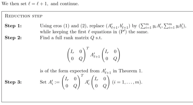
is infeasible for any α≥0,and weakly infeasible exactly when α= 0.
Since the constraint matrices are in FR(S2
+),we see that (3.2.1) is in the form of (Dref) ( and itself is a proof of infeasibility).
Supposeα= 0 and let
y1 =
0 0 0 1
, y2=
0 −1/2 −1/2 0
.
Then (y1, y2)∈FR(S+2), A∗(y1) = (0,0)T, A∗(y2) = (0,−1)T, so (y1, y2) proves that (3.2.1) is not strongly infeasible.
Classically, the set of right hand sides that make (D) weakly infeasible, is the frontier of A∗K∗ defined as the difference betweenA∗K∗ and its closure. In this case
front(A∗K∗) = clA∗S+2 \A∗S+2 = {(0, λ) : λ6= 0}.
For all such right hand sides a suitable (y1, y2) proves that (3.2.1) is not strongly infeasible.
In Section 3.7 we present our exact certificates of infeasibility and weak infeasibility of general conic LPs, and in Section 3.8 we describe the corresponding certificates for SDPs. We also present our geometric corollaries: an exact characterization of when the linear image of a closed convex cone is closed, an exact characterization ofnice cones(Pataki [29], Roshchina [40]), and bounds on how many constraints can be dropped from, or added to a (weakly) infeasible conic LP, while keeping its feasibility status. Note that when K∗ (and
K) is polyhedral, and (D) is infeasible, a single equality constraint obtained using eros and membership in K∗ proves infeasibility (by Farkas’ lemma). In the general case the number of necessary constraints is related to the length of the longest chain of faces inK. In Section 3.9 we define a natural class of weakly infeasible SDPs, and provide a simple algorithm to generate all instances in this class. In Section 3.10 we present a library of infeasible, and weakly infeasible SDPs, and our computational results. Section 3.11 concludes.
3.3 Literature Reviews
Facial reduction algorithms – see Borwein and Wolkowicz [11; 10], Waki and Muramatsu [49], and Pataki [30] – achieve exact duality between (P) and (D) by constructing a suitable smaller cone, say F, to replace K in (P), and to replace K∗ by F∗ (a larger cone) in (D).
Extended strong duals for semidefinite programs and generalizations – see Ramana [35], Klep and Schweighofer [20], Pataki [30] – use polynomially many extra variables and constraints. We note that Ramana’s dual relies on convex analysis, while Klep and Schweighofer’s uses ideas from algebraic geometry. The approaches of facial reduction and extended duals are related – see Ramana, Tun¸cel and Wolkowicz [36], and [30] for proofs of the correctness of Ramana’s dual relying on facial reduction algorithms. The paper [30] gen-eralizes Ramana’s dual to the context of conic LPs over nice cones. See P´olik and Terlaky [32] for a generalization of Ramana’s dual for conic LPs over homogeneous cones.
the strong conical hull intersection property. Pataki [27] gives necessary conditions, which subsume well known sufficient conditions, and are necessary and sufficient for a broad class of cones, callednice cones.
Borwein and Moors [8; 9] recently showed that the set of linear maps under which the image isnotclosed isσ-porous, i.e., it has Lebesgue measure zero, and is also small in terms of category. For characterizations of nice cones, see Pataki [29]; and Roshchina [40] for a proof that not all facially exposed cones are nice.
Elementary reformulation for SDPs – see Pataki [28] and Liu and Pataki [21] – use simple operations, as elementary row operations, to bring a semidefinite system into a form from which its status (as infeasibility) is trivial to read off. We refer to Lourenco et al [22] for an error-bound based reduction procedure to simplify weakly infeasible SDPs, and a proof that weakly infeasible SDPs contain another such system whose dimension is at most
n−1.We generalize this result in Theorem 12.
3.4 Notations and preliminaries
We assume throughout that the operator A is surjective. For x and y in the same Euclidean space we sometimes write x∗y forhx, yi.For a convex setC we denote its linear span, the orthogonal complement of its linear span, its closure, and relative interior by linC, C⊥,clC, and riC, respectively.
We define the dual cone of K as
K∗ = {y| hy, xi ≥0,∀x∈K},
and for convenience we set
We say that strong duality holds between (P) and (D) if their values agree and the latter is attained when finite. This is true when (P) is strictly feasible, i.e., when there isx∈Rm withb−Ax∈riK.
ForF, a convex subset ofKwe say thatF is afaceofK, ify, z ∈K, and 1/2(y+z)∈F
implies y, z∈F.
Definition 5. IfH is an affine subspace with H∩K 6=∅, then we call the smallest face of
K that containsH∩K the minimal cone of H∩K.
The traditional alternative system of (P) is
A∗y = 0
b∗y = −1
y ≥K∗ 0;
(Palt)
if it is feasible, then (P) is infeasible and we say that it is strongly infeasible.
For a nonnegative integer r we denote by Sr
+⊕ {0} the subset ofS+n (where n will be clear from the context) with psd upper leftr byr block, and the rest zero, and write
S+r ⊕ {0}=
⊕ 0 0 0
,(S+r ⊕ {0})∗ =
⊕ ×
× ×
(3.4.2)
where the × stand for matrix blocks with arbitrary elements. All faces of Sn
+ are of the form tT(Sr
+⊕0)twhere tis an invertible matrix [3; 26]. We write
Aut(K) = {T :Y →Y |Tis linear and invertible, T(K) =K} (3.4.3)
for the automorphism group of a closed convex coneK.
Definition 6. We say thatF1, . . . , Fkfaces ofKform achain of faces,ifF1)F2 )· · ·)Fk and we write `K for the length of the longest chain of faces inK.
For instance, `Sn
3.5 The properties of the facial reduction cone
In Lemma 2 we record relevant properties of FRk(K).Its proof is given in Appendix A. Lemma 2. Fork≥0 the following hold:
(1) FRk(K) is a convex cone.
(2) FRk(K) is only closed ifK is a subspace ork= 1.
(3) IfT ∈Aut(K),and (y1, . . . , yk)∈FRk(K) then
(T y1, . . . , T yk)∈FRk(K).
(4) IfC is another closed convex cone, then
FRk(K×C) = FRk(K)×FRk(C).
Precisely,
(y1, z1), . . . ,(yk+1, zk+1)
∈ F Rk(K×C) (3.5.4)
if and only if
y1, . . . , yk+1
∈FRk(K) and z1, . . . , zk+1
∈FRk(C). (3.5.5)
Proof of Lemmas 2 and 3
Proof of Lemma 2
ClaimIf C is a closed, convex cone and y, z∈C∗,then
C∩(y+z)⊥=C∩y⊥∩z⊥.
We let (y1, . . . , yk),(z1, . . . , zk)∈FRk(K),and for brevity, fori= 1, . . . , k we set
Ky,i = K∩y⊥1 ∩ · · · ∩y ⊥ i ,
Kz,i = K∩z1⊥∩ · · · ∩z⊥i ,
Ky+z,i = K∩(y1+z1)⊥∩ · · · ∩(yi+zi)⊥.
We first prove that for i= 1, . . . , k the relation
Ky+z,i = Ky,i∩Kz,i holds. (3.5.6)
Fori= 1 this follows from the Claim. Suppose now that (3.5.6) is true withi−1 in place of i.Then
yi ∈ Ky,i∗ −1 ⊆ (Ky,i−1∩Kz,i−1)∗ = Ky∗+z,i−1, (3.5.7)
where the first containment is by definition, the inclusion is trivial, and the equality is by using the induction hypothesis. Analogously,
zi ∈ Ky∗+z,i−1. (3.5.8)
Hence
where the first equation is trivial. The second follows since by (3.5.7) and (3.5.8) we can use the Claim withC =Ky+z,i−1, y=yi, z=zi. The third is by the inductive hypothesis, and the last is by definition. This completes the proof of (3.5.6).
Now we use (3.5.7), (3.5.8) and the convexity ofKy∗+z,i−1 to deduce that
yi+zi ∈Ky∗+z,i−1 holds fori= 1, . . . , k.
This completes the proof of (1).
Proof of (2) LetL=K∩ −K,assumeK 6=L,andk≥2.Let{y1i} ⊆riK∗, s.t. y1i→0. Then
K∩y⊥1i = L, ⇒ (K∩y1⊥i)∗ = L⊥ K∩0⊥ = K ⇒ (K∩0⊥)∗ = K∗.
Let y2 ∈ L⊥\K∗. (Such a y2 exists, since K∗ 6= L⊥.) Then (yi1, y2,0, . . . ,0) ∈ FRk(K), and it converges to (0, y2,0, . . . ,0)6∈FRk(K).
Proof of (3) Let us fix T ∈Aut(K) and letS be an arbitary set. Then we claim that
(T S)∗ = T−1S∗, (3.5.9)
(T S)⊥ = T−1S⊥, (3.5.10)
(K∩(T S)⊥)∗ = T(K∩S⊥)∗ (3.5.11)
hold. The first two statements are an easy calculation, and the third follows by
(K∩(T S)⊥)∗ = (K∩T−1S⊥)∗ = (T−1(K∩S⊥))∗ = T(K∩S⊥)∗,
where in the first equation we used (3.5.10), in the second equation we used T−1K = K
Now let (y1, . . . , yk) ∈ FRk(K), and Si = {y1, . . . , yi−1} for i = 1, . . . , k. Then by definition we have yi ∈ (K∩Si⊥)∗ and (3.5.11) implies
T yi ∈ (K∩(T Si)⊥)∗,
which completes the proof.
Proof of (4) The equivalence of (3.5.4) and of (3.5.5) is trivial fork= 0 so let us assume thatk≥1 and we proved it for 0, . . . , k−1.Statement (3.5.4) is equivalent to
(y1, z1), . . . ,(yk, zk)
∈ F Rk−1(K×C)
and
(yk+1, zk+1) ∈ (K×C)∩(y1, z1)⊥∩ · · · ∩(yk, zk)⊥
∗
. (3.5.12)
By the inductive hypothesis the set on the right hand side of (3.5.12) is
(K∩y⊥1 ∩ · · · ∩yk⊥)∗×(C∩z1⊥∩ · · · ∩z⊥k)∗,
and this completes the proof.
3.6 Facial reduction and strong duality for conic linear program
In this section we present a very simple facial reduction algorithm to findF, the minimal cone of the system
H∩K, (3.6.13)
whereHis an affine subspace withH∩K6=∅and our exact duals of (P) and of (D). While simple facial reduction algorithms are available, the convergence proof of Algorithm 1, with an upper bound on the number of steps, is particularly simple.
To start, we note that ifF is the minimal cone of (3.6.13) then H∩riF 6=∅(otherwise
then replacingK byF in (P) makes (P) strictly feasible, and keeps its feasible set the same. Hence if we also replaceK∗ byF∗ in (D) then strong duality holds between (P) and (D).
To illustrate this point, we consider the following example: Example 4. The optimal value of the SDP
sup x1
s.t. x1
0 1 0
1 0 0
0 0 0
+x2
0 0 1
0 1 0
1 0 0
1 0 0
0 0 0
0 0 0
(3.6.14)
is zero. Its usual SDP dual, in which we denote the dual matrix byy and its components by yij, is equivalent to
inf y11
s.t.
y11 1/2 −y22/2 1/2 y22 y23 −y22/2 y23 y33
0, (3.6.15)
which does not have a feasible solution withy11= 0 (in fact it has an unattained 0 infimum).
Since all slack matrices in (3.6.14) are contained in S1
+⊕0 and there is a slack matrix whose (1,1) element is positive, the minimal cone of this system is F = S1
+⊕0.If in the dual program we replace S3
+ by F∗ then the new dual attains with
y :=
0 1/2 0 1/2 0 0
0 0 0
∈ F∗ = ⊕ × × × × × × × × (3.6.16)
To construct the minimal cone we rely on the following classic theorem of the alternative (recallK∗\⊥=K∗\K⊥).
H∩riK =∅ ⇔H⊥∩K∗\⊥6=∅. (3.6.17)
Algorithm 1 repeatedly applies (3.6.17) to find F : Algorithm 1 Facial Reduction
Initialization: Let y0= 0, F0 =K, i= 1. while ∃yi ∈H⊥∩Fi∗\⊥−1 do
Choose such ayi. LetFi=Fi−1∩y⊥i . Leti=i+ 1.
end while
To analyze Algorithm 1 we need a definition:
Definition 7. Fork≥1 we say that (y1, . . . , yk)∈FRk(K) isstrict, if
yi ∈ (K∩y1⊥∩ · · · ∩y ⊥
i−1)∗\⊥fori= 1, . . . , k.
We say that it is pre-strictif (y1, . . . , yk−1) is strict.
If (y1, . . . , yk) is strict, then these vectors are linearly independent. Assuming that they are not, for some 1≤i≤k a contradiction follows:
yi ∈lin{y1, . . . , yi−1} ⊆ (K∩y1⊥∩ · · · ∩y⊥i−1)⊥.
Recall that `K is the length of the longest chain of faces in K (Definition 6). Theorem 3. The following hold:
(1) Ify1, . . . , yk are found by Algorithm 1, then (y1, . . . , yk)∈FRk(K) and