USING THE MULTI-STRING BURROW-WHEELER TRANSFORM FOR HIGH-THROUGHPUT SEQUENCE ANALYSIS
James Matthew Holt
A dissertation submitted to the faculty at the University of North Carolina at Chapel Hill in partial fulfillment of the requirements for the degree of Doctor of Philosophy in the Department of
Mathematics in the College of Arts and Sciences.
Chapel Hill 2016
Approved by:
Leonard McMillan
Jan Prins
Vladimir Jojic
Fernando Pardo-Manuel de Villena
c
ABSTRACT
James Matthew Holt: Using the Multi-String Burrow-Wheeler Transform for High-Throughput Sequence Analysis
(Under the direction of Leonard McMillan)
The throughput of sequencing technologies has created a bottleneck where raw sequence files
are stored in an un-indexed format on disk. Alignment to a reference genome is the most common
pre-processing method for indexing this data, but alignment requiresa priori knowledge of a reference
sequence, and often loses a significant amount of sequencing data due to biases. Sequencing data can
instead be stored in a lossless, compressed, indexed format using the multi-string Burrows Wheeler
Transform (BWT).
This dissertation introduces three algorithms that enable faster construction of the BWT for
sequencing datasets. The first two algorithms are a merge algorithm for merging two or more BWTs
into a single BWT and a merge-based divide-and-conquer algorithm that will construct a BWT
from any sequencing dataset. The third algorithm is an induced sorting algorithm that constructs
the BWT from any string collection and is well-suited for building BWTs of long-read sequencing
datasets. These algorithms are evaluated based on their efficiency and utility in constructing BWTs
of different types of sequencing data. This dissertation also introduces two applications of the BWT:
long-read error correction and a set of biologically motivated sequence search tools. The long-read
error correction is evaluated based on accuracy and efficiency of the correction.
Our analyses show that the BWT of almost all sequencing datasets can now be efficiently
constructed. Once constructed, we show that the BWT offers significant utility in performing fast
searches as well as fast and accurate long read corrections. Additionally, we highlight several use
This dissertation is dedicated to my wife Caroline for her unwavering support through graduate school and my son Luke for providing motivation
ACKNOWLEDGEMENTS
First and foremost, I would like to thank my savior Jesus Christ for providing me and my family
with all the things we have needed. Without him, I would not be where I am today.
I would also like to thank my advisor Leonard McMillan for his support and enthusiasm for
bioinformatics. I also want to thank the members of my committee Jan Prins, Vladimir Jojic,
Fernando Pardo-Manuel de Villena, and Yun Li for their support and constructive feedback. I wish
to thank past and present members of Computational Biology lab who have provided both help
and occasional lab entertainment: Leonard McMillan, Jeremy Wang, Catie Welsh, Shunping Huang,
Ping Fu, Katy Kao, Zhaoxi Zhang, Piyush Aggarwal, Seth Greenstein, Sebastian Sigmon, and
Anwica Kashfeen. I also wish to thank all of the members of the Systems Genetics group, especially
Fernando Pardo-Manuel de Villena and Andrew Parker Morgan for their numerous collaborations
and willingness to explain genetics.
I’d like to thank all of the members of the UNC Computer Science staff for their administrative
and technical assistance. Thank you to the NIH for the grants that have funded my education and
research at UNC. I also want to thank my mother Kim, father Barney, and sister Allison for all their
encouragement, support, and love for all of my life. Thank you to all my friends and family for the
fun, laughter, and motivation. I’d like to thank my son Luke for being a little bundle of joy. Finally,
I’d like to thank my wife Caroline for endless support and love throughout everything. Love you,
TABLE OF CONTENTS
LIST OF FIGURES . . . x
LIST OF TABLES . . . xi
CHAPTER 1: INTRODUCTION . . . 1
1.1 The computational bottleneck in bioinformatics . . . 1
1.2 Thesis statement . . . 3
1.3 Contributions . . . 3
1.4 Structure . . . 3
CHAPTER 2: BACKGROUND . . . 5
2.1 The suffix array . . . 5
2.2 The Burrows-Wheeler Transform . . . 5
2.3 The Full-text Minute-space index . . . 7
2.3.1 Retrieving a suffix . . . 8
2.3.2 Calculating suffix ranges . . . 10
2.3.3 Sampling the FM-index . . . 10
2.3.4 Application to bioinformatics . . . 11
2.4 The Multi-String Burrows-Wheeler Transform . . . 12
2.4.1 BWT functions on a string collection . . . 12
2.4.2 Representing De Bruijn graphs . . . 14
2.4.3 Application to bioinformatics . . . 14
CHAPTER 3: MERGING BURROWS-WHEELER TRANSFORMS . . . 17
3.1 Related work . . . 17
3.2 Approach . . . 18
3.3.1 Merge variables . . . 19
3.3.2 Iterations of the merge . . . 20
3.3.3 Convergence in the merge algorithm . . . 22
3.3.4 Generalizing the merge algorithm for more than two BWTs . . . 25
3.3.5 Asymptotic performance . . . 26
3.4 Results . . . 28
3.4.1 Merge times . . . 28
3.4.2 Compression . . . 28
3.4.3 Interleave storage . . . 34
3.5 Potential applications of merged BWTs . . . 34
CHAPTER 4: MULTI-STRING BWT CONSTRUCTION VIA MERGING . . . 36
4.1 Related work . . . 36
4.2 Approach . . . 37
4.3 Construction via merging . . . 38
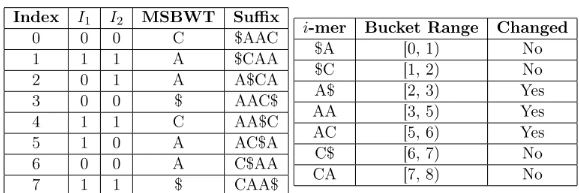
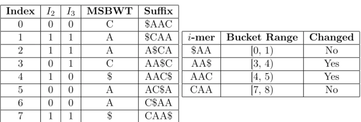
4.3.1 Tracking buckets . . . 38
4.3.2 Divide-and-conquer merge . . . 43
4.4 Results . . . 44
4.4.1 Dataset description . . . 44
4.4.2 Divide-and-conquer application . . . 46
4.4.3 Delayed tracking benefits . . . 47
4.4.4 Full construction times . . . 47
4.5 Final notes . . . 50
CHAPTER 5: MULTI-STRING BWT CONSTRUCTION VIA INDUCED SORT-ING . . . 52
5.1 Related work . . . 52
5.2 Approach . . . 55
5.3 Construction via induced sorting . . . 57
5.3.1 Computing the S* substring alphabet . . . 57
5.3.3 Inducing the BWT . . . 61
5.3.4 Asymptotic performance . . . 63
5.4 Results . . . 65
5.4.1 BWT construction tools . . . 65
5.4.2 Simulated datasets . . . 66
5.4.3 Long-read datasets . . . 68
5.4.4 Genome and transcriptome datasets . . . 70
5.5 Final notes . . . 70
CHAPTER 6: LONG READ CORRECTION VIA FM-INDEX QUERIES . . . . 72
6.1 Related work . . . 72
6.2 Approach . . . 74
6.3 Correction of long read sequences using BWTs . . . 75
6.3.1 The BWT and implicit De Bruijn graph . . . 75
6.3.2 Identification of weak regions . . . 76
6.3.3 Correction of weak regions . . . 76
6.3.4 Differences in the short and long passes . . . 77
6.4 Results . . . 81
6.4.1 Correction and alignment tools . . . 81
6.4.2 Data description . . . 82
6.4.3 FMLRC parameter selection . . . 82
6.4.4 Alignment-based results . . . 84
6.4.5 Performance . . . 86
6.5 Final notes . . . 86
CHAPTER 7: BWT-BASED WEB TOOLS . . . 89
7.1 Related work . . . 89
7.2 Approach . . . 90
7.3 Data description . . . 91
7.4 k-mer based query tools . . . 91
7.6 Reference based tools . . . 98
7.7 Targeted assembly tool . . . 102
7.8 Final notes . . . 104
CHAPTER 8: CONCLUSION . . . 109
8.1 Summary . . . 109
8.2 Future work . . . 110
APPENDIX A: MULTI-STRING BWT UTILITY SUITE . . . 113
A.1 Command line interface . . . 113
A.2 Python/Cython API . . . 114
A.3 BWT formats . . . 115
LIST OF FIGURES
2.1 Example de Bruijn graph . . . 15
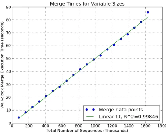
3.1 Merge execution times. . . 29
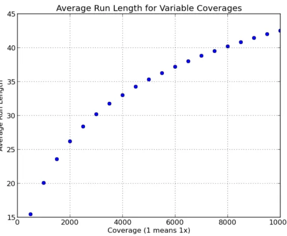
3.2 Average run length by coverage . . . 31
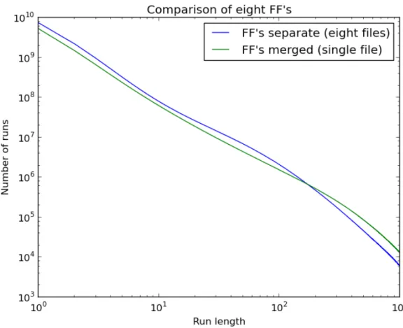
3.3 Run-length distributions in a merge . . . 33
4.1 Divide-and-conquer merge . . . 45
4.2 Divide-and-conquer merge implementation . . . 46
4.3 Tracking run-time comparison . . . 48
4.4 Tracking memory comparison . . . 49
5.1 BWT-IS example . . . 56
5.2 MSBWT-IS overview . . . 58
5.3 Performance - small simulated datasets . . . 67
5.4 Performance - large simulated datasets . . . 69
6.1 Examplek-mer graph . . . 79
6.2 ExampleK-mer graph . . . 80
7.1 K-mer lookup tool . . . 92
7.2 K-mer lookup tool with multiple alleles . . . 93
7.3 K-mer allele tool . . . 95
7.4 Mass query tool . . . 97
7.5 Batch query tool . . . 98
7.6 Reference based tool . . . 100
7.7 Reference based correction . . . 101
7.8 WSB/EiJ duplication example . . . 103
7.9 Egr3 de Bruijn graph . . . 105
LIST OF TABLES
2.1 Suffix array example . . . 6
2.2 BWT example . . . 6
2.3 FM-index example . . . 8
2.4 recoverSuffix(...) example . . . 9
2.5 getRange(...) example . . . 11
2.6 Multi-string BWT example . . . 13
2.7 recoverSuffix(...) string collection example . . . 13
3.1 Two-way merge example . . . 26
3.2 Three-way merge example . . . 27
3.3 Merge asymptotic performance . . . 27
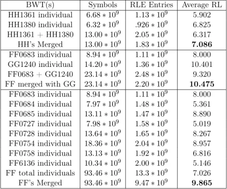
3.4 Compressibility of merges . . . 32
4.1 Bucket example - initial state . . . 40
4.2 Bucket example - iteration 1 . . . 41
4.3 Bucket example - iteration 2 . . . 41
4.4 Bucket example - iteration 3 . . . 42
4.5 Merge-based construction performance . . . 50
5.1 S* substring example - level 0 . . . 59
5.2 S* substring example - level 1 . . . 60
5.3 S* substring suffixes - level 1 . . . 62
5.4 Induced BWT - level 1 . . . 63
5.5 S* substring suffixes - level 0 . . . 64
5.6 Induced BWT - level 0 . . . 64
5.7 Long-read dataset performance . . . 70
5.8 Genome dataset performance . . . 70
6.1 Data summary . . . 82
6.3 Long read correction results . . . 85
CHAPTER 1
INTRODUCTION
1.1 The computational bottleneck in bioinformatics
The throughput of next generation sequencing (NGS) technologies has increased at such a rate
that it is now on the cusp of outpacing downstream computational and analysis pipelines [Kahn,
2011]. The result is a bottleneck where huge datasets are held on secondary storage (disk) while
awaiting processing. Raw sequence (ex. FASTQ) files, composed of sequence and quality strings, are
the most common intermediate piling up at this bottleneck. Moreover, the rapid development of new
analysis tools has led to a culture of archiving raw sequence files for reanalysis in the future. This
hoarding tradition reflects an entrenched notion that the costs of data generation far exceeds the
costs of analysis. The storage overhead of this bottleneck can be somewhat alleviated through the
use of compression. However, most analyses require additional computational stages to decompress
datasets prior to their use, which further impacts the throughput of subsequent analyses. This, in
turn, has led to the need for algorithms which can operate directly on compressed data [Loh et al.,
2012].
The goal of next generation sequencing is to read in sequences of DNA, RNA, or processed DNA
such that they can be analyzed. Generally speaking, these sequences are composed of long chains of
four different nucleotides that are commonly represented by four characters: A, C, G, and T. In
complex organisms, the strands of DNA (called chromosomes) can be millions of nucleotides long
leading to whole genomes that are billions of nucleotides long. Currently, NGS technologies are
not capable of directly reading these long strands of DNA. Instead, they rely on fragmenting the
sequence into smaller pieces and reading those smaller pieces using the sequencing technology. These
smaller reads are usually hundreds or thousands of nucleotides long and have an expected error
rate from the sequencing technology. A typical raw sequence file will include both the nucleotide
sequence read by the technology and a quality score indicating the confidence in each nucleotide in
Others have previously proposed representing the raw sequencing data using the Burrows Wheeler
Transform (BWT) and FM-index [Mantaci et al., 2005, Bauer et al., 2011, Cox et al., 2012a]. The
BWT is more compressible than raw sequencing data, and the FM-index is created in a way that is
suitable for direct queries by downstream tools even when the BWT is compressed. Furthermore,
the BWT is a lossless transform of the sequences that only needs to be computed once for any given
dataset. Once computed, the FM-index enables arbitrary, exact matching searches for k length
strings in O(k) steps. These searches can be used to count the frequency of the k length string and/or extract all sequenced reads that contain thek length string as a substring.
Despite the benefits of compression and arbitrary searches, there are relatively few efficient
algorithms for constructing the BWT of raw sequencing data. While many algorithms exist for
constructing the BWT of a single, long string, only a handful exist for constructing the BWT
of a string collection such as a sequencing dataset. The ones that do exist also tend to work
well for only a particular type of dataset. For example, the BCR algorithms [Bauer et al., 2011,
2013] work well for short, uniform length reads like those produced by an Illumina1 sequencer.
Unfortunately, the algorithm requires more computation time as the reads become longer, leading to
lengthy computations for long read sequencing datasets like those produced by PacBio2 or nanopore3
sequencers. This has created a barrier of entry for researchers who do not have efficient ways to
compute the BWT and FM-index for their datasets.
Once a BWT and FM-index are constructed, they can be applied as the underlying data structures
for accessing raw sequencing data, enabling methods that solve biological problems like de novo
assembly [Simpson and Durbin, 2010] or splice junction detection [Cox et al., 2012b]. Unfortunately,
it is not immediately obvious how to use the structures unless one is first familiar with the subroutines
used to compute FM-index queries. As a result, there is a second barrier of entry where researchers
are unsure how to query the data stored in a BWT and use it in a biologically meaningful way.
In this dissertation, three new algorithms for the multi-string BWT are introduced: a multi-string
BWT merge algorithm, a merge-based multi-string BWT construction algorithm, and an induced
1
http://www.illumina.com 2
sorting based multi-string BWT construction algorithm. These three methods are primarily geared
towards addressing the problem of efficiently computing BWTs of long read sequencing datasets.
This dissertation also describes two applications of the BWT and FM-index to addressing biological
problems: long-read sequence correction and sequence visualizations. Long-read sequence correction
is an automated process that reduces the noise caused by sequencing errors in long-read datasets,
enabling downstream analyses such asde novo assembly and alignment to operate on a cleaner set
of inputs. The sequence visualizations enable researchers to directly access raw sequence datasets
stored on a remote server while masking the complexities of the BWT and FM-index queries. These
tools provide a direct interface to the sequenced reads without losing information from a preprocess
like alignment or assembly. Since the BWT is a lossless transform that only need to be computed
and indexed once for a dataset, it enables researchers to focus their efforts on designing biologically
informative queries instead of repeatedly preprocessing the data.
1.2 Thesis statement
The multi-string Burrows-Wheeler Transform and associated FM-index are efficient data
struc-tures for storing and indexing raw sequencing data. By developing methods to build these strucstruc-tures
for different types of sequencing data, we enable alternate methods for solving biologically relevant
problems without loss of the underlying, raw sequence data.
1.3 Contributions
This dissertation introduces three main BWT algorithms: an algorithm for merging multiple
BWTs into a single BWT, a merge-based multi-string BWT construction algorithm, and an
induced-sorting based multi-string BWT construction algorithm. Both construction algorithms tend to be
better suited for long read sequencing datasets than other construction algorithms. This dissertation
also introduces two methods that use the BWT as an underlying data structure for querying a
sequence dataset: a long-read error correction method that uses the BWT and FM-index of a
short-read sequencing dataset and a collection of sequence-centric visualization tools for directly
accessing raw sequencing data through a BWT and FM-index.
1.4 Structure
Chapter 2 provides an overview and background of the BWT and FM-index. Chapter 3 describes
two algorithms for constructing multi-string BWTs of long-read sequencing datasets that respectively
use a merge-based approach and an induced sorting approach. Chapter 6 describes a method for
long-read error correction using the BWT of short-read sequencing datasets. Chapter 7 describes how
to use the BWT to create sequence-centric web tools for accessing and visualizing raw sequencing
CHAPTER 2
BACKGROUND
2.1 The suffix array
The suffix array is a data structure that enables searches for substrings in a single string [Manber
and Myers, 1993]. Let T be a string of length N that is terminated by a unique end-of-string
character, ‘$’, that is lexicographically smaller than all other symbols in T. One can naïvely
construct the suffix array ofT by first enumerating all of its suffixes,S0 =T[0 :N],S1 =T[1 :N], ..., SN−2 = T[N −2 : N], and SN−1 = T[N −1 : N], and then sorting them lexicographically. The suffix indices after the sort is the suffix array of T. While the suffix array is defined as the
list of suffix indices, it is often visually represented as the actual suffixes. Table 2.1 illustrates the
construction of the suffix array for the string “ALABAMA$".
The suffix array is a useful data structure primarily because it organizes similar substrings so
that they are adjacent to each other in the structure. Since suffix arrays represent a sorted list,
a standard binary search can be used to search for exact matching substrings within the text T.
Manber and Myers [1993] show that this binary search can be performed inO(k+log(N))time for a text of length N and a substring of lengthk.
The main disadvantage of a suffix array is the memory cost for storing the structure. The
array storesN values that are at most(N−1). As a result, the total storage cost of the array is O(N ∗log(N)) bits. For any long text, the size of the structure may be too large to fit in main memory. For example, the human genome is approximately three billion basepairs long, so the
suffix array for the human genome requires approximately 12 GB of memory. While this may not
be prohibitively large for modern computers, there are smaller structures that can perform faster
searches.
2.2 The Burrows-Wheeler Transform
Index Suffix Sorted Suffixes Suffix Array
0 ALABAMA$ $ 7
1 LABAMA$ A$ 6
2 ABAMA$ ABAMA$ 2
3 BAMA$ ALABAMA$ 0
4 AMA$ AMA$ 4
5 MA$ BAMA$ 3
6 A$ LABAMA$ 1
7 $ MA$ 5
Table 2.1: Suffix array example. This table demonstrates how to naïvely construct the suffix array for a string “ALABAMA$". First, list every suffix of the input string in the “Suffix" column. Then, lexicographically sort those suffixes in the “Sorted Suffixes" column. In the “Suffix Array" column, each sorted suffix is paired with its corresponding start index in our original string. For example, the suffix “$" starts at index 7 in “ALABAMA$", so the first value in the suffix array is 7. The array of numerical values forming this column is the suffix array for “ALABAMA$".
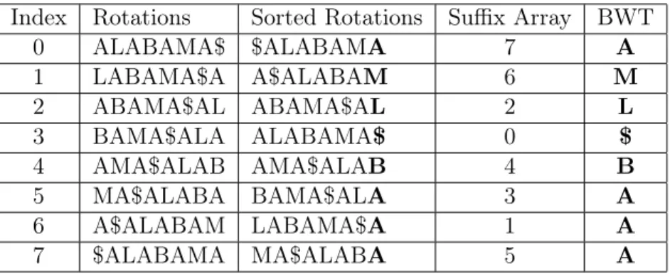
Index Rotations Sorted Rotations Suffix Array BWT
0 ALABAMA$ $ALABAMA 7 A
1 LABAMA$A A$ALABAM 6 M
2 ABAMA$AL ABAMA$AL 2 L
3 BAMA$ALA ALABAMA$ 0 $
4 AMA$ALAB AMA$ALAB 4 B
5 MA$ALABA BAMA$ALA 3 A
6 A$ALABAM LABAMA$A 1 A
7 $ALABAMA MA$ALABA 5 A
Table 2.2: BWT example. This table demonstrates how to naïvely construct the BWT for a string “ALABAMA$". First, list every rotation of the input string in the “Rotations" column. Then, lexicographically sort those rotations in the “Sorted Rotations" column. The values in the “BWT" column are generated by taking the corresponding sorted rotation and storing the symbol preceding that rotation (this is also the last symbol in the rotation, bolded for visual aid). Note that changing the suffixes to rotations has no effect on the values stored in the suffix array.
the permutation is directly related to a suffix array for the same string. Given a single string and its
suffix array, the BWT is a concatenation of the symbols preceding each suffix represented by the
suffix array. Alternatively, by representing the suffixes as rotations (cyclic suffixes), the BWT can be
thought of as a concatenation of the last characters in each rotation represented by the suffix array.
Thus the BWT implicitly represents a suffix array. Table 2.2 demonstrates how to construct the
BWT for the string “ALABAMA$".
The BWT enables compression because it tends to create long substrings of the same symbol
calledruns [Burrows and Wheeler, 1994]. This tendency to create long runs is largely due to its
the input, rotations that start with similar substrings will be adjacent in the array. Additionally, the
expectation is that similar substrings are preceded by the same symbol. Since the BWT is defined
as the concatenation of these predecessor symbols, the expectation is that long runs will occur in
the BWT when the same substring is repeated multiple times in the original string. For example,
consider a typical English text document. Words such as “the" will occur many times through the
document. In the suffix array, this will appear as suffixes starting with “he " and whose rotations end
with symbol ‘t’. As a result, there will likely be long runs of ‘t’ symbols caused by the prevalence of
the substring “the" in the text.
Given a BWT of a text, it can be compressed using run-length encoding [Burrows and Wheeler,
1994]. Wherever a run occurs in the BWT, the run can be replaced with a numerical value and
a single occurrence of the symbol that makes the run. For example, the string “ALABAMA$"
becomes BWT “AML$BAAA" which can be stored using run-length encoding as “AML$B3A". As
the length of runs in the BWT increases, the relative compression gained from run-length encoding
also increases.
2.3 The Full-text Minute-space index
While the BWT is an interesting data structure for compressing long texts, it is not inherently
searchable like the suffix array. However, the suffix array that is implicitly represented by the
BWT can be accessed through an auxiliary data structure called the Full-text Minute-space index
(FM-index) [Ferragina and Manzini, 2001]. The FM-index takes advantage of a relationship between the BWT and suffix array called the Last-to-First Mapping (LF-mapping) property [Ferragina and Manzini, 2001]. The LF-mapping property states that j-th occurrence of a symbol c in the
BWT (the Last column in a sorted rotation) corresponds in a 1-to-1 manner with the j-th suffix
that begins with symbol cin the suffix array (the First column in a sorted rotation). For example,
in Table 2.3, the first ‘B’ in the BWT occurs at index 0 and corresponds to the first suffix starting
with ‘B’ at index 4. Similarly, the second ‘B’ in the BWT occurs at index 1 and corresponds to
the second suffix starting with ‘B’ at index 5. The FM-index pre-calculates and stores these 1-to-1
relationships to enable fast access to the implicit suffix array.
Index Suffix Array BWT FM-index
$ A B
0 $ABABAB B 0 0 0
1 AB$ABAB B 0 0 1
2 ABAB$AB B 0 0 2
3 ABABAB$ $ 0 0 3
4 B$ABABA A 1 0 3
5 BAB$ABA A 1 1 3
6 BABAB$A A 1 2 3
Total — — 1 3 3
Offsets — — 0 1 4
Table 2.3: FM-index example. A sample BWT and FM-index for the string “ABABAB$". The sorted rotations from the suffix array are shown for visual aid. The FM-index, F, is shown on the far right. For index iand symbolc,F[i][c]is the number of occurrences of c beforeiin the BWT. Additionally, the last entry in the FM-index (labeled “Total") is the total number of times each symbol occurs in the BWT. These totals are used to derive an “Offsets" array, O, such that O[c]is the index of the first suffix in the suffix array that begins withc.
entire FM-index can be constructed in a linear pass over the BWT. InitializeF[0] to all zeros. For all ifrom0to N, copy F[i]into F[i+ 1] and increment onlyF[i+ 1][c]wherec=B[i]. Given this definition, the last entry in the FM-index is the total number of occurrences of all characters in the
BWT. These total counts are used to trivially calculate Offsets array,O, of length σ such that for
all c∈Σ,O[c]is the first suffix in the implicit suffix array that begins with c. Table 2.3 shows the BWT, FM-index, and Offsets for string “ABABAB$".
Given a BWT and FM-index, the corresponding suffix array can be implicitly accessed by
applying the LF-mapping property. Recall that the LF-mapping property relates the predecessor
symbol stored in the BWT to a particular suffix in the suffix array. As a result, substrings that are
contained within the suffix array can be accessed without explicitly storing the suffix array. There
are two key functions that use the FM-index to access the implicit suffix array in this way.
2.3.1 Retrieving a suffix
The first function is recoverSuffix(...) shown in Algorithm 1. The main idea behind this
algorithm is to repeatedly calculate the predecessor at a particular index in the BWT by using the
FM-index. Given an index i, lines 1-3 find the symbol preceding the implicit suffix at indexiand
the corresponding index of that suffix the BWT. In lines 4-7, the process of finding predecessor
symbols and suffixes is repeated until it returns to the original indexi. Since this calculation is done
symbols to obtain the actual suffix. A full example of this method is show in Table 2.4.
The time to find any given predecessor symbol and corresponding index in the BWT is O(1). Since this method recovers the entire suffix as a rotation, it will require a total of O(N) steps to recover the suffix of length N. Note that when this method is called on index 0 (the only suffix
starting with the end-of-string symbol ‘$’), the method returns a suffix that can be trivially shifted
to obtain the original text used to construct the BWT.
Data: BWTB, FM-indexF, Offsets O, index i
Result: The rotational suffix located at index iin the implicit suffix array
Function recoverSuffix(B, F, O, i)
1 c←B[i];
2 j ←O[c] +F[i][c]; 3 ret←c ;
4 while i6=j do 5 c←B[j];
6 j ←O[c] +F[j][c]; 7 ret.append(c) ;
end
8 return reverse(ret) ;
Algorithm 1:Given a BWT and FM-index, this function accesses the implicit suffix array through a reverse traversal of the BWT. Line 1 retrieves the symbol preceding the suffix at index i in the implicit suffix array. Line 2 calculates the index of the suffix corresponding to that symbol and stores it inj. Line 3 saves the symbol as part of a string. Since the suffixes are cyclic (i.e. rotations) by the BWT definition, lines 4-7 repeats the retrieval of predecessors until it reaches the original indexi, at which point the algorithm has cycled through the entire suffix in reverse order. Since the symbols are discovered in reverse order, the final step is to reverse the entire string in line 8 before it is returned. An example execution of this process is shown in Table 2.4.
Variable Lines 1-3 Loop 1 Loop 2 Loop 3 Loop 4 Loop 5 Loop 6
c B A B A B A $
j 4 1 5 2 6 3 0
ret B BA BAB BABA BABAB BABABA BABABA$
Table 2.4: recoverSuffix(...) example. This table shows the state of variables in the
2.3.2 Calculating suffix ranges
The second function is getRange(...) shown in Algorithm 2. Given a substringp of length k
(called a k-mer), this method solves for a range in the implicit suffix array such that all suffixes in the range share thek-mer prefix p. The base case is the empty string range defined as [0, N) for a BWT of length N (lines 1-3). In the loop, symbols from the substring are retrieved in reverse
order (lines 4-5). For iteration i∈[1, k], the symbol is used to calculate a new range corresponding to the i-mer suffix of p. At the end of iteration i, the values [l, h) store the range of suffixes in the implicit suffix array that are prefixed by the i-mer substring p[k−i:k). In other words, the algorithm implicitly pre-pends symbols to the empty string range until it obtains the substring p. A
full example of this method is show in Table 2.5.
As with recoverSuffix(...), this method traverses the values stored in the BWT in reverse
order. For any given range, a symbol can be implicitly pre-pended to that range in O(1) steps (lines 5-7). Thus, the range for any arbitraryk-mer can be solved inO(k) steps. Additionally, the count or frequency of a k-mer can be derived trivially as the length of the range,(h−l).
Data: BWTB, FM-indexF, Offsets O, Prefix p
Result: The range of suffixes [l, h) in the suffix array that have the prefixp
Function getRange(B, F, O, p)
1 k←len(p); 2 l←0; 3 h←len(B); 4 for i∈[1..k]do 5 c←p[k−i]; 6 l←O[c] +F[l][c]; 7 h←O[c] +F[h][c];
end
8 return (l, h);
Algorithm 2: Given a BWT of length N and FM-index, this function calculates the range of indices in the BWT corresponding to suffixes in the implicit suffix array that have a particular prefixp of lengthk. It starts with the full range[0, N) and implicitly prepends characters from p in reverse order. In other words, the method calculates the range corresponding to suffixes p[k−1 :k),p[k−2 :k), ...,p[1 :k), and finallyp. This method takes advantage of the LF-mapping property stored in the FM-index to solve for any givenk-length substring (or k-mer) inO(k)steps. An example execution of this process is shown in Table 2.5.
2.3.3 Sampling the FM-index
While the FM-index is useful for the methods described above, it requires a significant amount
Variable Lines 1-2 Loop 1 Loop 2 Loop 3 Loop 4
c — B A B A
l 0 4 1 5 2
h 7 7 4 7 4
partial substring “" B AB BAB ABAB
Table 2.5: getRange(...) example. This table shows the state of variables in thegetRange(...)
function of Algorithm 2 when called using the BWT, FM-index, and Offset array from Table 2.3 andp=“ABAB". The algorithm starts with the full range (l, h= [0,7)) corresponding to the empty string. The range is modified such that symbols are implicitly prepended to the substring (shown in the partial substring row) with each execution of the main loop. The correct range for suffixes of the substring p are solved in reverse order, and the final execution of the loop solves the range[2,4) for the full substring “ABAB".
FM-index requiresO(N σ)integer values. Even for a restricted genomic alphabet, this is too large to be practical.
Fortunately, there is a relatively easy way to sample the FM-index to reduce storage costs by
sampling the FM-index [Ferragina and Manzini, 2001]. Given BWT B and FM-index F, recall
that the values in F[i+ 1] were defined earlier based on the values stored atF[i] andB[i]. As a result, given an FM-index entry at index i < j, the BWT can be linearly traversed to calculate the
FM-index entry at index j. If the FM-index is sampled such that every s-th entry is stored, the
total memory requirements of the FM-index reduces to O(N σs ). Note that this comes at a cost of increasing the time to get any particular FM-index to O(s)due to the linear traversal ofB.
2.3.4 Application to bioinformatics
One of the most common ways to index short-read datasets is through a process called alignment.
In alignment, the goal is to match a sequencing read (a short string) to a reference genome (a
much longer string) such that the edit distance (number of symbol changes, insertions, or deletions)
between the read and the reference are minimized. In this way, each read is indexed by a position in
the reference genome. In DNA-seq alignment, there are often millions or billions of reads that need
to be aligned to the reference genome.
Two prominent alignment tools, BWA [Li and Durbin, 2009] and Bowtie [Langmead et al., 2009],
use the BWT and FM-index to quickly align reads. Both methods first construct a BWT and
FM-index of the reference genome. Additionally, there is some amount of bookkeeping (i.e. a suffix
array) required to store the location of some or all of the suffixes in the original reference genome.
seeds). The tools then search for exact matches to thek-mer seeds in the BWT. If a seed is found,
the methods identify the location of the seed in the original reference genome and perform a more
extensive local alignment that allows for inexact matching of the full read to the reference. In general,
these methods are quite fast because they use theO(k)search algorithm made possible by the BWT and FM-index. Additionally, the method has been adapted for RNA-seq alignment in at least one
publicly available tool, Tophat [Trapnell et al., 2009].
2.4 The Multi-String Burrows-Wheeler Transform
Thus far, the BWT has only been discussed in the context of a single input string. However, there
are many reasons one might wish to encode a string collection. For example, a reference genome for
a complex organism often has multiple strings where each string represents a chromosome for the
organism. The BWT of a single string was well-defined because there was only one end-of-string
symbol. However, with multiple strings, the relative ordering of the symbols can be permuted leading
to many different (and conflicting) orderings of the strings.
While there are many definitions, we adopt the multi-string BWT definition used by Bauer
et al. [2011]. In general, this version defines the lexicographic order of end-of-string characters
as the lexicographic order of the strings in the collection. In other words, for two strings si
and sj in the collection that are terminated with end-of-string symbols $i and $j respectively,
(si < sj) ⇐⇒ ($i<$j). This defines an unambiguous order of all suffixes represented by the BWT. Given the above definition, one can naïvely construct the BWT of a string collection in a method
very similar to the naïve construction method for a single string. First, all rotations of all strings
are generated. Then, all rotations are sorted lexicographically. Finally, the predecessor symbols to
each sorted rotation are concatenated and stored as the BWT for the collection. Additionally, the
FM-index for a multi-string BWT is calculated in the exact same way as a single-string BWT. A
simple example of a BWT and FM-index for a string collection is shown in Table 2.6.
2.4.1 BWT functions on a string collection
Both recoverSuffix(...) and getRange(...) functions can be used unchanged on the BWT
and FM-index of a string collection. Additionally, the chosen definition of a multi-string BWT enables
the extraction of individual strings in the collection using therecoverSuffix(...) function. Recall
that the definition orders the ‘$’ character by lexicographic order of the strings in the collection. As a
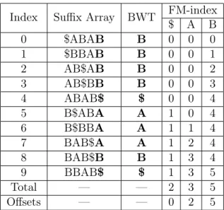
Index Suffix Array BWT FM-index
$ A B
0 $ABAB B 0 0 0
1 $BBAB B 0 0 1
2 AB$AB B 0 0 2
3 AB$BB B 0 0 3
4 ABAB$ $ 0 0 4
5 B$ABA A 1 0 4
6 B$BBA A 1 1 4
7 BAB$A A 1 2 4
8 BAB$B B 1 3 4
9 BBAB$ $ 1 3 5
Total — — 2 3 5
Offsets — — 0 2 5
Table 2.6: Multi-string BWT example. A sample BWT and FM-index for the string collection, ABAB$, BBAB$. The rotations of each string in the collection are sorted to create the suffix array. The BWT is the concatenation of predecessor symbols (bolded). The FM-index F is defined as before for indexiand symbols csuch that F[i][c]is the number of occurrences ofc beforeiin the BWT. Note that the order of suffixes beginning with ‘$’ corresponds exactly to the lexicographic ordering of the strings in the collection.
Variable Lines 1-3 Loop 1 Loop 2 Loop 3 Loop 4
c B A B A $
j 5 2 7 4 0
ret B BA BAB BABA BABA$
Table 2.7: recoverSuffix(...) string collection example. This table shows the state of variables in the recoverSuffix(...) function of Algorithm 1 when called using the BWT, FM-index, and Offset array from Table 2.6 andi= 0. Note that this traversal never “jumps" into the suffixes created by other strings in the collection. After the final loop, ret is reversed and the lexicographically smallest rotation (“$ABAB") corresponding to the lexicographically smallest string in the collection (“ABAB$") is returned.
traversal are guaranteed to be from string si. In other words, in a correct traversal, it is impossible
to “jump" from one string in the collection to a different string in the collection. Given this result,
callingrecoverSuffix(...) will only return the rotation for a specific string. An example of the
recoverSuffix(...) method run on a BWT of a string collection is shown in Table 2.7.
The getRange(...) functionality is largely the same as before. However, instead of searching for
occurrences of a substring in one string, this function will solve for all occurrences of the substring in
all strings in the collection. Again, the count or frequency of a particular substring in the collection
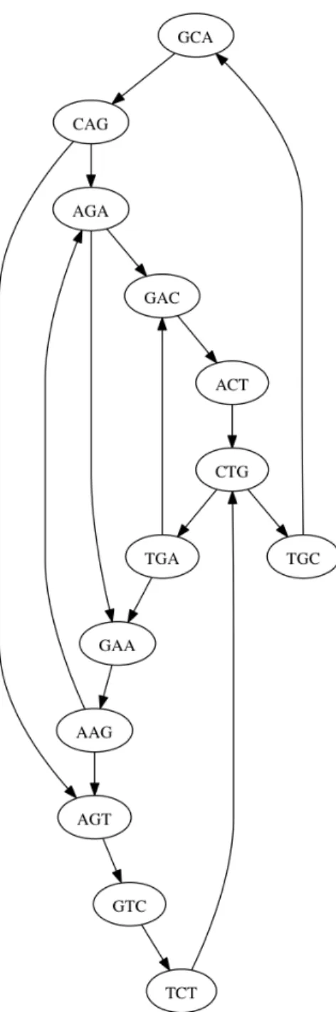
2.4.2 Representing De Bruijn graphs
One way of traversing the information in a string collection is to use an auxiliary data structure
called the de Bruijn graph. In a de Bruijn graph, every k-length substring from the collection is
represented as a single node [Bruijn, 1946]. The graph also has directed edges drawn between nodes
such that the (k−1) suffix of the source node is identical to the(k−1) prefix of the destination node [Bruijn, 1946]. This graph representation reduces the long strings into shorter substrings of a
fixed length, allowing for algorithms to then intelligently traverse the graph to perform tasks like
de novo assembly [Simpson and Durbin, 2010] or read correction [Salmela and Rivals, 2014]. An
example de Bruijn graph containing two strings is shown in Figure 2.1.
Generally speaking, de Bruijn graphs are usually explicitly stored for a fixed, smallkusing either
a hash based method or a bloom filter [Chikhi and Rizk, 2013]. Additionally, these graphs are often
pruned such that k-mers with low frequency are removed from the graph. The BWT and FM-index
can actually be used to implicitly represent a de Bruijn for all sizes of k up to the length of the
stored strings. When a node in the graph needs to be accessed, thegetRange(...) function (see
Section 2.3.2) can be used to retrieve the k-mer frequency. If the k-mer frequency is above the
pruning threshold, then thek-mer node is considered present in the de Bruijn graph, otherwise it is
absent. Additionally, since thegetRange(...) function is not constrained to a particular k size,
this method can be used to represent all de Bruijn graphs for a string collection without needing to
explicitly calculate or store the graph.
2.4.3 Application to bioinformatics
A multi-string BWT can be used to replace the concatenation method for building a BWT of
the reference genome. However, when built for a reference genome, these two structures are actually
very similar simply because the number of strings in a reference genome is relatively small. Most of
the implicit suffixes will be in the same order and the ones that are not will likely have little to no
effect on the alignment process. Instead, others have previously proposed storing raw sequencing
data in a BWT [Mantaci et al., 2005, Bauer et al., 2011, Cox et al., 2012a]. There are two main
benefits to applying the BWT to raw sequencing data: compression and indexing.
First, recall that BWTs achieve compression through the process of run-length encoding and that
those runs are formed due to repeated substrings within the text. In sequencing data, one source
typically amplified prior to sequencing leading to many copies of the genome that is often referred
to as the coverage. However, sequencing technologies are not perfect and generate errors during
the sequencing process. These errors work against the compression of BWTs essentially by creating
random noise that can break runs apart and reduce the compression ratio.
The second main benefit is that by building an FM-index, the sequencing data becomes searchable.
In the context of functions already discussed, this means that there are methods to count the frequency
of any given k-mer and to extract every read from a sequencing data that contains a particular
substring for further analysis. Additionally, the FM-index of genomic strings is relatively small
because the alphabet is generally limited to six characters (‘$’, ‘A’, ‘C’, ‘G’, ‘N’, and ‘T’). BWTs of
sequencing datasets have been used by other authors for splice junction detection [Cox et al., 2012b]
CHAPTER 3
MERGING BURROWS-WHEELER TRANSFORMS
The BWT and FM-index are useful data structures for analyzing genomic sequencing data. They
enable compression of the data while simultaneously indexing it for downstream analysis. While
there are several methods for constructing the BWT of single strings or string collections, there
are few methods for incrementally adding strings to a BWT without recalculating the entire data
structure.
In this chapter, we address the problem of merging two or more BWTs such that the result is a
BWT containing the combined string collections from each input BWT [Holt and McMillan, 2014a].
Additionally, we require the strings in the resulting BWT to be annotated such that the origin of
each string (in terms of which input it came from) can be identified later. The reasons for merging
include adding new information to an existing dataset (more data from a sequencer), combining
different datasets for comparative analysis, and improving compression.
3.1 Related work
Other researchers have addressed problems related to merging BWTs, and three of these are
of particular interest. The first is actually a BWT construction algorithm which incrementally
constructs a BWT in blocks and then merges those blocks together [Ferragina et al., 2012]. The
algorithm creates partial BWTs in memory. These partial BWTs are not truly independent BWTs
because they reference suffixes not included in the partial BWT (they either were processed previously
or will be processed later). The partial BWTs are then merged into a final BWT on disk by comparing
the suffixes either implicitly or explicitly depending on the location of the suffixes in the partial
BWTs. Their algorithm is primarily applicable to constructing a BWT of very long strings. However,
it could be adapted for merging by inserting one string at a time as if the string collection were
one long string. The memory overhead of the modified algorithm requires reconstituting the string
collections for all but one of the inputs (the one used as the starting point), and then iteratively
The second algorithm is also a BWT construction algorithm that creates a multi-string BWT by
incrementally inserting a single symbol from each string “columnwise" until all symbols are added to
the multi-string BWT [Bauer et al., 2011, 2013]. Given a finished BWT, they also describe how to
add new strings to the BWT using this algorithm. This algorithm could be adapted to solve the
proposed BWT merging problem by keeping one input in the BWT format and decoding all of the
other inputs into their original string collections. Then, their construction algorithm would merge
each collection into the BWT in this “columnwise" manner. As with the first algorithm, the main
issue with this approach is storage overhead of decoding each BWT into its original string collection.
The third algorithm is a suffix array merge algorithm which computes the combined suffix array
for two inputs [Sirén, 2009]. These suffix arrays are actually represented as two multi-string BWTs.
The algorithm searches for the strings of one collection in the other BWT to determine a proper
interleave of the first suffix array into the second. Once the interleave is calculated, the merged BWT
is trivially assembled. The algorithm requires an auxiliary index (such as the FM-index) to support
searching. As discussed in Section 2.3, the memory overhead of an unsampled FM-index isO(N)
where N is length of the BWT. While sub-sampling of the FM-index reduces this memory cost, it
will also impact search performance. Moreover, this algorithm is ill-suited to multiple datasets (more
than two) to merge. In this case, the algorithm performs multiple merges until only one dataset
remains.
Our algorithm merges two or more BWTs directly without any search index or the need to
reconstitute any string or suffix of the input BWTs. The only auxiliary data structures required
are two interleave arrays which identify the input source of each symbol in the final result, so the
only auxiliary data structures used by the algorithm are stored as part of the result. The merging is
accomplished by permuting the interleaves of the input BWTs, which is proven to be equivalent to a
radix sort [Knuth, 1998] over the suffixes of the string collections.
3.2 Approach
Similar to previous approaches [Bauer et al., 2011, 2013, Ferragina et al., 2012, Sirén, 2009],
our approach also takes advantage of the fact that a BWT implicitly represents a suffix array (see
Section 2.2). Intuitively, when two or more BWTs are merged, the relative orders of the suffixes
within each original BWT do not change because they must maintain a stable sort order in the
interleaving of the original input BWTs such that the result implicitly represents a combined, fully
sorted suffix array [Sirén, 2009].
Our merging algorithm is an iterative method that converges to the correct interleave of two or
more BWTs [Holt and McMillan, 2014a]. It starts by assuming the interleave is just a concatenation
of BWTs. Then, in each iteration, it adjusts the current interleave during a pass through the BWT
inputs. Each iteration acts as a single pass of an implicit radix-sort [Knuth, 1998] that corrects
the interleave. After the first iteration, the first symbols of each suffix (‘A’, ‘C’, ‘G’, etc.) are
grouped. After the second iteration, all identical di-mer suffixes (‘AA’, ‘AC’, ‘AG’, etc.) are grouped.
Eventually, the interleave converges to the correct solution, which is detected by two consecutive
iterations resulting in identical interleaves (in other words, the interleave did not change). Finally,
the two BWTs are merged based on the converged interleave and the result is stored as a single BWT.
This method can be extended to merge any number of BWTs simultaneously in O(LCS∗N)time where LCS is the longest common substring between any two BWTs andN is the total combined
length of the merged output.
3.3 The merge algorithm 3.3.1 Merge variables
Let two input BWTs, B0 andB1, be defined over a finite alphabet,Σ, with lexicographically ordered symbols $ < c1 < c2 < ... < cσ. A string is defined as a series of k symbols from this alphabet terminated with a special end-of-string symbol, ‘$’. LetS be a collection of such strings, S ={s1, s2, ..., sm}. All BWTs are assumed to be in the form described in Section 2.4 such that any string can be reconstituted by prepending the predecessors repeatedly until the starting index is
reached (each string forms a cycle in the BWT). In a single pass through all input BWTs, the total
number of occurrences of each symbol is counted and used to calculate a list of offsets into the final
BWT indicating the first suffix in the output starting with each symbol. These counts and offsets
are a tiny subset of the FM-index (see Section 2.3), but for the unknown output BWT, rather than
the known input BWTs.
Overall, the goal of the algorithm is to construct an interleave of the two input BWTs such
that the implicit, combined suffix array is in sorted order. We call this interleave the “correct"
in the merged output. It begins by constructing an initial interleave of the input BWTs that is
simply a concatenation of the inputs. Then, a series of iterations are performed on the interleave.
Each iteration acts like one pass of a most-significant-symbol radix sort over the implicit suffix array
represented by the interleaved BWTs. After one iteration, the interleave will be such that all suffixes
are lexicographically sorted by their first symbol. After two iterations, the interleave will be such
that all suffixes are lexicographically sorted by their first two symbols. The third is the first three
symbols. These iterations will continue until there is no change in the interleave, indicating that the
implicit suffix array has converged to a correct interleave.
Given two BWTs, B0 =bwt(S0) andB1 =bwt(S1), of lengthm andn respectively, note that the target result, B2 = bwt({S0, S1}), can be trivially constructed if the interleave of B0 and B1 is known. As such, the primary goal of our proposed method is to calculate this interleave. Let I
be auxiliary array called the interleave that is a series of zeroes and ones of length (m+n) such that a zero corresponds to a symbol in B2 originating fromB0 and a one corresponds to a symbol
originating from B1. There are exactly m zeroes and exactlynones in I. As the merge algorithm
progresses, this interleave will be corrected until it converges to the final interleave. ThisI array is
similar to the interleave array described in Sirén [2009].
Let totals array T be a list of numbers such that for each symbol c inΣ,T[c] =count(c, B0) + count(c, B1). In short,T is a total combined count of each symbol in the two BWTs. Additionally, let offsets array O be defined for each symbolcsuch that O[c] is the position of the first suffix in the merged BWT,B2, that starts withc, which can be calculated by adding theT values for all symbols
lexicographically beforec. Note that this is equivalent to the offsets component of the FM-index for
the final merged BWT (see Section 2.3).
3.3.2 Iterations of the merge
The main iteration function of the merge algorithm, mergeIter(...), is defined in Algorithm 3.
Repeated calls to this procedure converge to the correct interleaving ofB0 and B1 resulting inB2.
To prove this claim, we first show that a correct interleave will not change as a result of this function.
Lemma 3.3.1. Given a correct interleaveI, of two BWTs,B0 and B1, into a single BWTB2, and
the offsets array O, for each symbol c ∈ Σ into B2, then mergeIter(I, B0, B1, O) will return the
Data: I - the current interleave of B0 andB1;B0 - the first BWT to merge;B1 - the second BWT to merge;O - for eachc∈Σ, O[c] is the position of the first suffix starting withc in the merged BWT
Result: IN ext - the new interleave
Function mergeIter(I, B0,B1, O)
// initial conditions
1 INext ←[null]∗len(I); 2 currentP os0←0; 3 currentP os1←0; 4 tempIndex←O;
// iterate through each bit value in I 5 forall theb∈I do
// b is a bit representing the input BWT
6 if b= 0 then
7 c←B0[currentP os0];
8 currentP os0←currentP os0 + 1;
else
9 c←B1[currentP os1];
10 currentP os1←currentP os1 + 1;
end
// copy b into the next position for symbol c 11 IN extP os←tempIndex[c];
12 IN ext[IN extP os]←b;
// update the tempIndex to match the FM-index
13 tempIndex[c]←tempIndex[c] + 1;
end
return IN ext;
Proof: This lemma follows from the properties of a BWT. The lemma assumes that the ordering of interleaveI results in a correct BWT B2, for a collection of strings S2 ={S0, S1}. In the initial condition, the current positions are both 0 and the tempIndex value corresponds to the offsets
into the merged BWT array. First, it’s easily noted that after each iteration, i = 1..(m +n), currentP os0 +currentP os1 = i. This is because as i increments, one of the currentP os values is also incremented at the end of the loop. Additionally, if given an FM-index F and offsets O
for the BWT represented by I, note thattempIndex=O+F[i] after each iteration. Before any iterations, thetempIndex is set to O andF[0]is all zeros, so the initial condition holds. With each iteration i, a symbol c is determined by the interleave and used to identify the indextempIndex[c]
to increment such that the conditiontempIndex=O+F[i]holds at each iteration. Finally, after each iteration, one value of IN ext is changed corresponding to the current tempIndex[c]. Since tempIndex[c] = O +F[i], this implies that the LF-mapping property (see Section 2.3) of the FM-index also holds, so each iteration is effectively setting IN ext[tempIndex[c]] =I[tempIndex[c]]. After doing this for all values binI, the algorithm has set every value inIN extto its corresponding
value inI. Alternatively, if there exists a position, j, such thatIN ext[j]6=I[j], then the original assumption thatI is a correct interleave must be false because there is at least one position where
the implied FM-index causes a suffix originating from B0 to have a predecessor symbol originating
fromB1 (or vice-versa) which cannot happen in a correct BWT.
The point of Lemma 3.3.1 is that given an interleaveIi, its covergence can be verified by executing
mergeIter(...) once and comparing the resulting interleaveIi+1 with the original input interleave
Ii. IfIi =Ii+1, then the interleave has converged on the correct solution.
3.3.3 Convergence in the merge algorithm
The function,mergeIter(...), is also a convenient subroutine that performs one iteration in the
merge of two BWTs. To apply this function for a full merge requires simple setup and an outer-loop
to test for convergence. The pseudocode for thebwtMerge(...) operation is presented in Algorithm
4.
As described in Section 2.2, the BWT implicitly represents a sorted suffix array. The BWT can
also generate partial suffixes or the firstisymbols (i-mer prefix) of the suffix. We will refer to these
asi-suffixes. Given a BWT, the symbols of the BWT can be sorted using a radix sort to recover
Data: B0 - the first BWT to merge;B1 - the second BWT to merge;Σ- lexicographically ordered valid symbols in the BWTs
Result: The correct interleave ofB0 and B1 to form a new BWT
Function bwtMerge(B0, B1, Σ)
// initial pass to calculate offsets O 1 of f ←0;
2 forall thec∈Σdo
3 T[c]←count(c, B0)+count(c, B1); 4 O[c]←of f;
5 of f ←of f+T[c];
end
// initialize the ret array to zeroes followed by ones
6 I ←null;
7 ret←[0]∗len(B0) + [1]∗len(B1); 8 while I 6=ret do
// copy the old interleave and re-iterate
9 I ←ret;
10 ret←mergeIter(I, B0, B1, O);
end
return ret;
Algorithm 4: This function will calculate the interleave for merging two BWTs into a single output BWT. The algorithm repeatedly callsmergeIter(...) until it detects convergence in the interleave. Once converged, the resulting BWT can be trivially created using the output interleave.
sorted again using only the prepended BWT characters, all 2-suffixes in the BWT are recovered in
lexicographic ordering. If this process is repeated foriiterations, alli-suffixes in the BWT can be
recovered. This is equivalent to doing a least significant symbol radix sort of all i-suffixes in the
suffix array. Since the algorithm is sorting the prefixes of the suffixes by increasing the prefix length
i, it is really performing a most-significant-symbol radix sort on the full suffixes in the suffix array.
Each iteration of the while loop in bwtMerge(...) is equivalent to performing an iteration
of the most-significant-symbol radix sort on the full suffixes. The I array indicates the current
interleave of symbols at the start of an iteration. Then, the interleave bits are copied into the next
available location for their corresponding symbol using the FM-index values stored in tempIndex.
With each iteration in the loop, the sorting of suffixes is extended by one symbol untilI converges to
a correct interleave. Note that the actual suffixes are never explicitly reconstructed or stored. In the
example executions in Tables 3.1 and 3.2, the suffixes are shown after each iteration for illustration
only. The final merged BWT is created trivially using the interleave from bwtMerge(...).
come before all ones, afteri executions of mergeIter(...), all corresponding suffixes in the suffix
array implied byIi are stably sorted up to their first isymbols.
Proof: Using induction, consider the initial condition, i= 0. In this base case, all 0-suffixes are identical (empty string) and the ordering is all zeros followed by all ones. Now, consider
iteration (i+ 1) where the interleaving,Ii, is a stable sort of the firstisymbols of the suffixes of the corresponding BWTs. In the next iteration, the algorithm performs a pass over Ii retrieving the
corresponding predecessor symbol for each bit inIi. If two suffixes have different start symbols, then
those suffixes are automatically ordered correctly because each will be placed into the appropriate bin
for that symbol. As a property of the radix sort, all(i+ 1)-suffixes starting with the same symbol,c, are placed sequentially in the output in lexicographical ordering. Given that thei-suffixes are already
stably sorted, if the symbol cis found at two indices, x andy where x < y, then the corresponding
(i+ 1)-suffixes must be of the form cX andcY whereX is ani-suffix that lexicographically precedes the other i-suffix Y. This implies that the corresponding (i+ 1)-suffixes are also in sorted order in the new interleave Ii+1.
Theorem 3.3.3. Given that the longest common substring of two string collections stored in separate BWTs,B0 and B1, is of lengthk, and that the initial interleave,I0, is a single series of zeros followed
by ones, then thebwtMerge(...) algorithm will converge ink+ 1 or fewer iterations. Additionally, this convergence can be detected by iterating until interleave Ii stops changing.
Proof: Using Lemma 3.3.2, it’s known that after k+ 1 iterations, all (k+ 1)-suffixes will be lexicographically sorted. If the longest common substring (LCS) is of lengthk, then it follows that
after k+ 1 iterations the suffixes will be sorted up to their first(k+ 1)symbols. This means that further iterations will not change the sort order of the suffixes and that the interleave has converged.
Additionally, we know from Lemma 3.3.1 that convergence can be detected (i.e. the interleave can
be verified as correct) through an additional iteration.
Given that the combined size of the two input BWTs isN =n+m, this algorithm usesO(N)
bits of additional memory due to the creation of two interleave arrays I andIN ext. Assuming a
fixed alphabet, all other variables are constant sized. For practical purposes, all large arrays (B0,
B1) are actually stored on disk due to their size.
L, the algorithm will converge after at most (L+ 1)iterations. Additionally, this algorithm does allow for variable length strings. In fact, it is completely unaware of the string lengths present in
either BWT. However, the one caveat to Theorem 3.3.3 is the determination of LCS when the
input strings are of variable length. In some instances, there are string collections that can result in
iterations up to (2∗L+ 1) iterations due to the contents of the strings. The reason for this is the cyclic nature of strings in the BWT and the similarity between two BWTs. Consider two strings
‘AA$’ and ‘AAA$’. At first glance, theLCS= 3, ‘AA$’. However, because of the cyclic nature of the strings when represented in a BWT, the trueLCS = 5, ‘AA$AA’, which can be generated by starting from the first symbol in the first string and the second symbol in the second string and
cycling back through when there are no more symbols. For the real-data experiments presented in
this chapter, all strings were of identical length, so this caveat wasn’t an issue even in the presence
of identical strings in each input BWT.
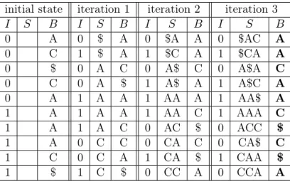
An example of an entire execution of bwtMerge(...) is shown in Table 3.1. For this basic
example, only two single-string BWTs were used in the merge. Iteration 0 represents the initial
condition and all subsequent iterations are the result from executing themergeIter(...) function
once. After three iterations, the algorithm has converged and verified the convergence.
3.3.4 Generalizing the merge algorithm for more than two BWTs
Until now, the algorithm has only been discussed and demonstrated using exactly two input
BWTs and a bit-vector to distinguish the originating BWT for each position in the merged BWT.
A basic extension of this technique repeatedly merges f input BWTs according to any binary tree
resulting in a single merged BWT at the tree’s root. This requires f−1merges. However, the faster way is to extend theI array to multiple bits allowing for multiple BWTs to be merged simultaneously.
For example, a byte array supports the merging of up to 256 multi-string BWTs simultaneously.
Given f input BWTs, the above proofs can be extended by starting with an initial I0 consisted
of a series of 0’s, series of 1’s, ..., series of f −1’s as the initial condition and an initial offsets calculated in a pass over allf inputs. Additionally, variables corresponding to a specific BWT (such
as B0,currentP os1, etc.) can be condensed into arrays of lengthf that can be indexed by the interleave value, b, at each position. Then, the algorithm can iterate as before until convergence
is reached. This algorithm extension allows for an arbitrary number of multi-string BWTs to be
initial state iteration 1 iteration 2 iteration 3
I S B I S B I S B I S B
0 A 0 $ A 0 $A A 0 $AC A
0 C 1 $ A 1 $C A 1 $CA A
0 $ 0 A C 0 A$ C 0 A$A C
0 C 0 A $ 1 A$ A 1 A$C A
0 A 1 A A 1 AA A 1 AA$ A
1 A 1 A A 1 AA C 1 AAA C
1 A 1 A C 0 AC $ 0 ACC $
1 A 0 C C 0 CA C 0 CA$ C
1 C 0 C A 1 CA $ 1 CAA $
1 $ 1 C $ 0 CC A 0 CCA A
Table 3.1: Two-way merge example. The above table shows the state after each iteration, i, for merging two BWTs each containing one string, “ACCA$" and “CAAA$" respectively. Their respective starting BWT strings are “AC$CA" and “AAAC$" which are shown in their concatenated initial state in the left most columns. At each iteration, the table shows the interleave,I, thei-suffixes,S, and what the merged BWT,B, is with that interleave. After the first iteration, there are three bins of zeroes followed by ones representing the threei-suffixes of length one: ‘$’, ‘A’, and ‘C’. The second iteration puts all 2-suffixes in their correct bins. After iteration 2, the algorithm has converged to the correct solution early. Iteration 3 will detect no change in the interleave, and the merged BWT in bold is stored as the final solution. Note that in each iterationi, thei-suffixes are in sorted order and alli-suffix bins containing both zeroes and ones have all zeros before all ones.
of this extension is shown in Table 3.2.
The merged BWT is a complete interleave of the multiple BWTs into a single dataset. Since
distinguishing the source of a particular BWT symbol may be important, the final interleave array
Ii can be stored as an auxiliary component to the merged BWT. Alternatively, if only the source of
a particular string (as opposed to each individual suffix) is required, the length of theI array can be
truncated as described in Section 3.4.3. This allows for a merged BWT to differentiate the original
source BWT for a particular string in later analyses.
3.3.5 Asymptotic performance
We summarize the algorithmic complexities for merging two BWTs in Table 3.3. Notice that the
performance of this algorithm is not directly affected by string length or the number of strings in
either BWT. For a constantN, increasing string length and decreasing the number of strings will
not affect run time unless there is also an increase in theLCS between the two BWTs. Furthermore,
the memory and disk requirements for this algorithm are relatively low. In memory, the algorithm
initial state iteration 1 iteration 2 iteration 3 iteration 4
I S B I S B I S B I S B I S B
0 C 0 $ C 0 $A C 0 $AC C 0 $ACA C
0 C 1 $ C 2 $A A 2 $AC A 2 $ACC A
0 $ 2 $ A 1 $C C 1 $CA C 1 $CAA C
0 A 0 A C 2 A$ C 2 A$A C 2 A$AC C
0 A 0 A $ 1 AA C 1 AAC C 1 AAC$ C
1 C 1 A C 0 AC C 0 AC$ C 0 AC$A C
1 C 1 A A 0 AC $ 1 AC$ A 1 AC$C A
1 A 2 A C 1 AC A 0 ACA $ 0 ACAC $
1 A 2 A $ 2 AC $ 2 ACC $ 2 ACCA $
1 $ 0 C A 0 C$ A 0 C$A A 0 C$AC A
2 A 0 C A 1 C$ A 1 C$C A 1 C$CA A
2 C 1 C A 0 CA A 2 CA$ C 2 CA$A C
2 $ 1 C $ 1 CA $ 1 CAA $ 1 CAAC $
2 C 2 C C 2 CA C 0 CAC A 0 CAC$ A
2 A 2 C A 2 CC A 2 CCA A 2 CCA$ A
Table 3.2: Three way merge example. The above table shows the state after each iteration, i, for merging three BWTs, each containing one string: “ACAC$", “CAAC$", and “ACCA$" respectively. Their respective starting BWT strings are “CC$AA", “CCAA$", and “AC$CA". At each iteration, the table shows the interleave, I, the i-suffix, S, and what the merged BWT, B, is with that interleave. Each iteration corrects the suffixes by one symbol which can be seen in theS columns of each iteration. After three iterations, the ordering is correct. Iteration 4 detects convergence of the interleave and the resulting BWT is shown in bold on the far right.
CPU time O(LCS∗N)
Max Memory bits O(N) - Two Interleaves
Disk I/O bits
O(LCS∗N ∗log(σ))- Input BWTs O(N ∗log(σ))- Output Merged BWT
O(N) - Output Final Interleave
it only writesO(N ∗log(σ))bits to disk.
3.4 Results 3.4.1 Merge times
The asymptotic runtime for the merge algorithm is O(LCS∗N). We developed a Cython implementation of the merge algorithm to test the actual performance on genomic datasets. First,
we performed an experiment using real reads from mouse data provided by the Sanger Institute1.
We chose two samples, WSB/EiJ and CAST/EiJ, to use for the merge. From these samples, we
extracted all reads from each dataset that were aligned to the mitochondria (the reason for this
choice becomes apparent in Section 3.4.2). The annotated mouse mitochondria is approximately
16,299 base pairs long. Between the two samples, there were over 1.6 million reads where each
read was 100 basepairs long (over 10,000x coverage combined). We sampled reads from each set
proportionally, created separate BWTs (one for WSB/EiJ, one for CAST/EiJ), and performed a
merge of the two BWTs. The results of the merge execution times with respect to the total number
of input sequences (reads) are shown in Figure 3.1. In these sampled datasets, the LCS term of
the expected run-time is essentially constant at LCS= 101, the read length. As a result, there is a linear relationship between the total number of sequences that are merged and the total wall clock
time to perform the merge.
3.4.2 Compression
One motivation for merging BWTs is to improve the compression. As discussed in Section 2.2,
the BWT was proposed as a method for data compression because it tends to create long runs of
repeated symbols that can be used by many compression schemes [Burrows and Wheeler, 1994]. The
reason long runs form is that the BWT has a tendency to cluster similar suffixes together, and there
is an expectation that those patterns have the same predecessor symbol (the value actually stored
in the BWT). Therefore, if the two input BWTs to a merge contain similar substrings, then the
compression should increase due to the ability to form longer runs. The redundancy of genomic
sequencing data results from two factors: the datasets themselves are individually over-sampled and
the genomes of distinct organisms tend to share genomic features reflecting a common origin.
1