5098.pdf

(1)

Insights into RNA structure by melding experiment and computation

Christine Elizabeth Hajdin

A dissertation submitted to the faculty of the University of North Carolina at Chapel Hill in partial fulfillment of the requirements for the degree of Doctor of Philosophy in

Department of Chemistry.

Chapel Hill 2013

(2)

ABSTRACT

CHRISTINE ELIZABETH HAJDIN: Insights into RNA structure by melding experiment and computation

(Under the direction of Kevin Weeks)

(3)

(4)

List of Tables

Table 2.1: Prediction accuracies as a function of algorithm and SHAPE

information. ...17 Table 2.2: Energy penalty per in-line pseudoknotted helix of length n. ...21

Table 2.3: ShapeKnots run times as a function of RNA length. ...26

Table 2.4: Prediction accuracies for seven RNA folding algorithms (following

(11)

List of Figures

Figure 1.1: Overview of SHAPE mechanism ...5

Figure 1.2: Simple pseudoknot motif in RNA. ...7

Figure 2.1: Overview of pseudoknot structure model and entropic penalty

terms. ...20

Figure 2.2: Representative ShapeKnots structure prediction for the SAM I

riboswitch. ...23

Figure 2.3: Optimization of the ∆G°SHAPE and ∆G°PK parameters (in kcal/mol)

by jackknifing. ...25

Figure 2.4: Summary of predictions for four H-type pseudoknots. ...32

Figure 2.5: Prediction summaries for two large, pseudoknot-containing RNAs. ...34

Figure 2.6: Representative examples in which ShapeKnots avoids

false-positive (top) or false-negative (bottom) pseudoknot predictions. ...35

Figure 2.7: Prediction summary for RNase P RNA. ...37

Figure 3.1: Predicted pseudoknots in HIV-1. ...58

Figure 3.2: Mutual information distribution for all base-pairing conformations

in the HIV-1 genome. ...60

Figure 3.3: LNA binding confirms predicted HIV-1 pseudoknots. ...62

Figure 3.4: Activities of HIV-1 mutants confirm importance of nucleotides in

predicted pseudoknots. ...63

Figure 3.5: Effects of mutations on SHAPE reactivities. ...65

Figure 4.1: Shannon entropies values over the HIV-1 genome. ...80

Figure 4.2: Distribution of the Shannon entropies from no SHAPE and

(12)

Figure 4.3: Identifying single nucleotide offsets in helices. ...84

Figure 4.4: Predicting Shannon entropies with pseudoknots. ...87

Figure 4.5: 5S E. coli no SHAPE, 1M7 and differential SHAPE ...89

Figure 4.6: 16S and 23S rRNA no SHAPE and 1M7 SHAPE predictions and

superimposed Shannon entropies ...91

Figure 4.7: Signal Recognition Particle 1M7 and differential SHAPE

predictions ...93

Figure 4.8: Shannon entropy calculations for small RNA predictions. ...95

Figure 4.9: Shannon entropy calculations for large RNA predictions. ...97

Figure 5.1: SHAPE-directed secondary structure model of the 16S rRNA

compared to the conventional model. ...111

Figure 5.2: SHAPE-directed structural models of small refolded regions ...112

Figure 5.3: The structure for the region between nucleotides 920-1410

predicted by DMD based on SHAPE data. ...113

Figure 5.4: SHAPE-directed structure refined using PHENIX for the region

between nucleotides 920-1410. ...114

Figure 6.1: Comparison of an accepted RNA structure with modeled tertiary

structures as a function of RMSD similarity. ...124

Figure 6.2: Replica exchange DMD simulations as a function of starting state

and of enforcing native base pairing. ...129

Figure 6.3: Distributions of decoy structures. ...130

Figure 6.4: Dependence of radius of gyration on chain length for compact

RNAs with higher-order tertiary structure interactions. ...132

(13)

Figure 6.7: Significance (p-value) analysis for RNA tertiary structure

(14)

List of Abbreviations

1M6 - 1-methyl-6-nitroisatoic anhydride 1M7 - 1-methyl-7-nitroisatoic anhydride di-GMP –diguanylate

DIS – Dimer initiation site

DMD - Discrete molecular dynamics DNA – Deoxyribonucleic acid GDT – Global distance test HCV - Hepatitis C virus

HIV-1 – Human immunodeficiency virus type 1 INF – Interaction network fidelity

IRES – Internal ribosome entry site LNA – Locked nucleic acid

NE – Nested helices NL – Inline helices

NMIA - N-methylisatoic anhydride NMR - Nuclear magnetic resonance MFE – Minimum free energy

mRNA – Messenger ribo-nucleic acid PBS – Primer binding site

PreQ1- Pre-queuosine

(15)

RNA – Ribo-nucleic acid RNase P – Ribonuclease P RRE – Rev response element

rRNA – Ribosomal ribo-nucleic acid SAM-I – S’adenosyl methionine

SARS – Severe acute respiratory syndrome

SHAPE - Selective 2'OH acylation analyzed by primer extension SRP – Signal recognition particle

SS – Single stranded

(16)

1. Chapter 1: Introduction

1.1RNA structure and function

Although ribonucleic acid (RNA) is often dismissed as a passive component of translation, RNA plays keys roles in viruses and cells. For example, viral RNAs, like the Human immunodeficiency virus type 1 (HIV-1) RNA, form important elements of structure essential for viral replication and transcription1_{. Riboswitch RNAs, like the} thiamine pyrophosphate (TPP) riboswitch, regulate cellular function2-4 and ribosomal RNAs are critical to translation. For instance the 16S and 23S rRNA found in E. coli

form the main structural component of the ribosome and coordinate between the mRNA, the tRNA and the elongating amino acid chain5, 6.

The ability of RNA to perform these multiple diverse functions depends on its capacity to form distinct structures. Identifying these distinct RNA structures is critical to understanding and characterizing the role of RNA in cells and viruses.

(17)

like the signal recognition particle (SRP)10, lysine riboswitch11, and even the 16S rRNA 12, 13_.

Despite the advancements of X-ray crystallography, it is not suitable for every RNA. To accurately identify a tertiary structure, the RNA must be able to form a well-ordered crystal. Without a well-well-ordered crystal, the diffraction data becomes ‘fuzzy’ and it is hard to model the electron density. Crystallization, or the act of making an RNA crystal, is a difficult and time-consuming process. Success depends on the specific RNA being tested, the concentration of different components in the solution, the pH, and the flexibility of the RNA. To aid in the crystallization process, and increase the stability of the RNA, high concentrations of proteins, ligands and other stabilizing elements are added. These conditions can perturb the RNA structure and shift it away from its lowest energy state which is adopted in solution13-15_

1.2Using computational algorithms to determine RNA structure

Due to the disadvantages of traditional structure probing techniques, computational algorithms have been developed as a useful alternative for RNA structure determination. However, predicting the tertiary structure of an RNA directly from a linear sequence is a difficult challenge. An important first step in this process is to determine the secondary structure.

(18)

with all motifs in a structure is summed to identify the energy of a potential structure. The potential structures are then sorted by their energy and the “correct” structure is identified to be the lowest energy structure. These MFE algorithms, classically called the mFold class of algorithms18, tend to work well for small RNAs, but suffer from inaccuracies due to incomplete energy rules and an inability to correctly rank structures with similar energies, (see Chapter 2) so do not work well for long or complicated RNAs.

Heuristic algorithms work in a similar fashion to MFE algorithms, but attempt to redefine energy rules by supplementing additional constraints from known structures19, 20. These constraints are implemented into the program using a series of fit equations that are optimized against known RNAs. These algorithms tend to work well for small RNAs that can be accurately fit with a small number of equations and parameters. However, the complexity of large RNAs requires additional equations and constraints. Since the number of known large RNA structures is small and biased toward those that are stable enough for crystallography, it results in over-optimized fits to a few RNAs.

Partition function algorithms use statistical characterizations of the equilibrium ensemble of RNA to determine secondary structures21, 22. They function by calculating the base pairing probability of each base pair combination in an RNA and then use this information to rank order potential structures. Like traditional MFE algorithms, partition function algorithms employ classic rules from thermodynamics to assign probabilities. As in the MFE algorithm, this tends to work well for small RNAs, but is not accurate for larger RNAs.

(19)

maintained when bases in the pair are mutated. For example, if one serotype of a virus has a predicted CG base pair, co-variation would be observed if in another serotype there is an AU pair in the same relative position. When a large number of homologous sequences are known and there is great variability in the sequences, this method, can provide accurate RNA secondary structures. Many structures have been solved by this method such as the 16S rRNA24, 25. However, if there are not a large number of sequences known, few base pairs can be correctly identified.

1.3Using SHAPE data to refine structural predictions

Previously, work demonstrated how incorporating experimental SHAPE data can help to improve the accuracy of computational algorithms26. SHAPE allows for the differentiation of single-stranded and base-paired nucleotides27 (Figure 1.1). The technique works by chemically foot-printing an RNA using a SHAPE reagent. This molecule preferentially reacts with single-stranded nucleotides, creating bulky 2’-O-adducts. These adducts can be probed using a reverse transcriptase, which dissociates when it encounters the 2’-O-adduct. This creates a series of cDNAs whose lengths correspond to the position of modification and whose abundance corresponds to the degree of modification. These cDNAs are resolved using capillary electrophoresis and aligned to a sequencing ladder27_{. After integration, background subtraction from a} no-reagent control reaction, and further data processing the end result is a SHAPE reactivity profile (Figure 1.1).

(20)

Figure 1.1: Overview of SHAPE mechanism

A) Schematic of SHAPE reagent (1M7) reacting with RNA. The SHAPE reagent preferentially reacts with single stranded nucleotides forming bulky 2’-O-adducts. These adducts can be detected using capillary electrophoresis.

B) After data processing, the SHAPE data can be viewed as a SHAPE reactivity profile. The profile plots the nucleotide sequence along the x-axis and the SHAPE reactivities along the y-axis. The reactivates are colored so that very highly reactive nucleotides (> 0.85) are colored red, highly reactivity orange (between 0.4 and 0.85), and lowly reactive (< 0.4) are colored black.

C) When the SHAPE data is superimposed on an RNA structure, single stranded nucleotides are usually red or orange indicating highly flexible and base paired nucleotides are colored back, indicating highly constrained.

(RNA)_constrained

OH 2’

(RNA)_flexible

OH 2’

2’-O-adduct

N O

O O

NO2

(RNA)

2' O H N O 1M7

NO2 0

1.0

5 10 15 20 25

0.7

0.3

CCC GG

U A

C G

G C

U

10

U G_C _GU ₃₀

G C

A U

G C

U

A G A

20

5'

3'

0 1.0

5 10 15 20 25 30

0.85

0.4

Highly Reactive

Un-reactive A)

(21)

sampling space and increase the accuracy of prediction. When this method was incorporated into a secondary structure prediction algorithm, RNAstructure, and applied to the 16S rRNA and 23S rRNA, the accuracy of the prediction of structure for these RNAs increased by more than 20% over a traditional mFold class algorithm 26.

1.4Challenges of prediction algorithms

The RNAstructure algorithm provided a critical first step in refining traditional dynamic programming, but despite its advances, RNAstructure still had several deficiencies. For instance, none of the traditional RNAstructure predictions allows for the prediction of pseudoknots. Pseudoknots form when the loop region of a helix base pairs to another place in a RNA structure. Figure 1.2 shows the secondary structure of a simple pseudoknot on a traditional secondary structure plot and on a circleplot. A circleplot plots the sequence of the RNA around the outside of the circle and base pairs as lines running through the circle. Pseudoknots are easily identified on circleplots because they form a cross-hatching pattern. Pseudoknot motifs are relatively rare, but often occur in key functional areas, such as the pseudoknot near the 5’ end of HIV-1 that allows for frame shifting28, and the central pseudoknot in the SAMI riboswitch29 necessary for ligand binding. Because of their biological importance, there is a need to confidently identify pseudoknots in RNA secondary structures30, 31_.

(22)

Figure 1.2: Simple pseudoknot motif in RNA.

On the left, the pseudoknot is shown on a traditional secondary structure plot. On the right, the pseudoknot is shown on a circleplot. Circleplots plot the sequence of the RNA around the circumference of the circle; lines running through the circle represent base pairs. Pseudoknots are easy to identify because they create a cross hatching pattern.

C CC GG

U A

C G

G C

U

10

U G_C U_G ₃₀

G C

A U

G C

U

A G A

20

5'

3'

Simple H-type pseudoknot

Pseudoknot

C

1 _{C C}

U

C

G

U 10

U

G

C

G

AG

UC

C

G

20 GG

A

G

U

C

U

C

G

30 U

A

G

A

(23)

key hypotheses to be made. Conversely, identifying a poorly supported structure allows incorrect hypotheses to be avoided. Lastly, previous work has generally focused on using SHAPE data to understand secondary structure predictions. To obtain a full understanding of RNA structure, we must eventually target tertiary structures.

1.5Research Overview

In this work, I sought to modify current algorithms to increase prediction accuracy and better understand RNA structure. My focus has been on finding techniques to include pseudoknots using SHAPE data in secondary structure predictions, and identifying methods to calculate the accuracy of structure predictions.

In Chapter 2, I discuss how we created a secondary structure prediction algorithm, ShapeKnots, which more accurately incorporates SHAPE reactivities and predicts pseudoknots. By incorporating these features, I show that the accuracy of prediction increases 30% over classic mFold class algorithms to reach 94% accuracy. In Chapter 3, I discuss how I can use the ShapeKnots algorithm to identify pseudoknots in HIV-1. I show that when tested in virio, these pseudoknots are critical to the replication of the HIV-1. In Chapter 4, I discuss how I can determine the accuracy of secondary structure prediction by calculating the Shannon entropy from a modified partition function.

(24)

use the central limit theorem to identify a useful metric for categorizing the success of tertiary structure predictions. This metric, denoted the “q value”, can be used to evaluate tertiary structure prediction quality.

1.6Perspective

(25)

1.7References

1. Frankel, A.D. & Young, J.A. HIV-1: fifteen proteins and an RNA. Annu Rev

Biochem67, 1-25 (1998).

2. Serganov, A., Polonskaia, A., Phan, A.T., Breaker, R.R. & Patel, D.J. Structural basis for gene regulation by a thiamine pyrophosphate-sensing riboswitch. Nature

441, 1167-1171 (2006).

3. Bocobza, S. et al. Riboswitch-dependent gene regulation and its evolution in the plant kingdom. Genes Dev21, 2874-2879 (2007).

4. Kubodera, T. et al. Thiamine-regulated gene expression of Aspergillus oryzae thiA requires splicing of the intron containing a riboswitch-like domain in the 5'-UTR. FEBS Lett555, 516-520 (2003).

5. Traub, P. & Nomura, M. Structure and function of E. coli ribosomes. V. Reconstitution of functionally active 30S ribosomal particles from RNA and proteins. Proc Natl Acad Sci U S A59, 777-784 (1968).

6. Shajani, Z., Sykes, M.T. & Williamson, J.R. Assembly of bacterial ribosomes.

Annu Rev Biochem80, 501-526 (2011).

7. Wilkinson, K.A. et al. High-throughput SHAPE analysis reveals structures in HIV-1 genomic RNA strongly conserved across distinct biological states. PLoS Biol6, e96 (2008).

8. Mooers, B.H. Crystallographic studies of DNA and RNA. Methods 47, 168-176 (2009).

9. Smyth, M.S. & Martin, J.H. x ray crystallography. Mol Pathol53, 8-14 (2000). 10. Hainzl, T., Huang, S. & Sauer-Eriksson, A.E. Structure of the SRP19 RNA

complex and implications for signal recognition particle assembly. Nature 417, 767-771 (2002).

11. Garst, A.D., Heroux, A., Rambo, R.P. & Batey, R.T. Crystal structure of the lysine riboswitch regulatory mRNA element. Journal of Biological Chemistry

283, 22347-22351 (2008).

12. Dunkle, J.A., Xiong, L., Mankin, A.S. & Cate, J.H. Structures of the Escherichia coli ribosome with antibiotics bound near the peptidyl transferase center explain spectra of drug action. Proc Natl Acad Sci U S A107, 17152-17157 (2010). 13. Sagi, I. et al. Crystallography of ribosomes: attempts at decorating the ribosomal

(26)

14. Lu, J., Li, N.S., Sengupta, R.N. & Piccirilli, J.A. Synthesis and biochemical application of 2'-O-methyl-3'-thioguanosine as a probe to explore group I intron catalysis. Bioorg Med Chem16, 5754-5760 (2008).

15. Egli, M. & Pallan, P.S. Insights from crystallographic studies into the structural and pairing properties of nucleic acid analogs and chemically modified DNA and RNA oligonucleotides. Annu Rev Biophys Biomol Struct36, 281-305 (2007). 16. Zhang, S.J. et al. RhesusBase: a knowledgebase for the monkey research

community. Nucleic Acids Res41, D892-905 (2013).

17. Tian, B. et al. Expanded CUG repeat RNAs form hairpins that activate the double-stranded RNA-dependent protein kinase PKR. Rna6, 79-87 (2000).

18. Zuker, M. Mfold web server for nucleic acid folding and hybridization prediction.

Nucleic Acids Res31, 3406-3415 (2003).

19. Westhof, E., Masquida, B. & Jaeger, L. RNA tectonics: towards RNA design.

Fold Des1, R78-88 (1996).

20. Ren, J., Rastegari, B., Condon, A. & Hoos, H.H. HotKnots: heuristic prediction of RNA secondary structures including pseudoknots. Rna11, 1494-1504 (2005). 21. Vreede, F.T., Chan, A.Y., Sharps, J. & Fodor, E. Mechanisms and functional

implications of the degradation of host RNA polymerase II in influenza virus infected cells. Virology396, 125-134 (2010).

22. Dong, H., Ding, L., Yan, F., Ji, H. & Ju, H. The use of polyethylenimine-grafted graphene nanoribbon for cellular delivery of locked nucleic acid modified molecular beacon for recognition of microRNA. Biomaterials 32, 3875-3882 (2011).

23. Eddy, S.R. & Durbin, R. RNA sequence analysis using covariance models.

Nucleic Acids Res22, 2079-2088 (1994).

24. Tocilj, A. et al. The small ribosomal subunit from Thermus thermophilus at 4.5 A resolution: pattern fittings and the identification of a functional site. Proc Natl

Acad Sci U S A96, 14252-14257 (1999).

25. Schluenzen, F. et al. Structure of functionally activated small ribosomal subunit at 3.3 angstroms resolution. Cell102, 615-623 (2000).

(27)

28. Gaudin, C. et al. Structure of the RNA signal essential for translational frameshifting in HIV-1. J Mol Biol349, 1024-1035 (2005).

29. Montange, R.K. & Batey, R.T. Structure of the S-adenosylmethionine riboswitch regulatory mRNA element. Nature441, 1172-1175 (2006).

30. Brierley, I., Gilbert, R.J. & Pennell, S. RNA pseudoknots and the regulation of protein synthesis. Biochemical Society transactions36, 684-689 (2008).

31. Brierley, I., Pennell, S. & Gilbert, R.J. Viral RNA pseudoknots: versatile motifs in gene expression and replication. Nat Rev Microbiol5, 598-610 (2007).

32. Ding, F. et al. Ab initio RNA folding by discrete molecular dynamics: from structure prediction to folding mechanisms. Rna14, 1164-1173 (2008).

33. Woese, C.R., Gutell, R., Gupta, R. & Noller, H.F. Detailed analysis of the higher-order structure of 16S-like ribosomal ribonucleic acids. Microbiological reviews

(28)

2. Chapter 2: ShapeKnots: accurate RNA secondary structure

predictions, including pseudoknots

2.1Introduction

2.1.1RNA structure and function.

RNA constitutes the central information conduit in biology1_{. Information is}

encoded in an RNA molecule at two levels: in its primary sequence and in its ability to form higher-order secondary and tertiary structures. Nearly all RNAs can fold to form some secondary structure and, in many RNAs, highly structured regions encode important regulatory motifs. Such structured regulatory elements can be comprised of canonical base pairs but may also feature specialized and distinctive RNA structures. Among the best characterized of these specialized structures are RNA pseudoknots. Pseudoknots are relatively rare but occur overwhelmingly in functionally important regions of RNA2-4_{. For example, all of the large catalytic RNAs contain pseudoknots}5, 6_;

roughly two-thirds of the known classes of riboswitches contain pseudoknots that appear to be essential for ligand binding and gene regulatory functions7_{; and pseudoknots occur}

prominently in the regulatory elements that viruses use to usurp cellular metabolism3_.

(29)

2.1.2Pseudoknots in RNA structure predictions.

Pseudoknots are excluded from the most widely employed algorithms used to model RNA secondary structure8_{. This exclusion is based on the challenge of}

incorporating the pseudoknot structure into the efficient dynamic programming algorithm used in the most popular secondary structure prediction approaches and because of the additional computational effort required. The prediction of lowest free energy structures with pseudoknots is NP-complete9_{, which means that lowest free energy structure cannot}

be solved as a function of sequence length in polynomial time. In addition, allowing pseudoknots greatly increases the number of (incorrect) helices possible and tends to reduce secondary structure prediction accuracies, even for RNAs that include pseudoknots. Current algorithms also have high false positive rates for pseudoknot prediction, necessitating extensive follow-up testing and analysis of proposed structures. Pseudoknot prediction is challenging, in part, for the same reasons that RNA secondary structure prediction is difficult. First, energy models for loops are incomplete because they extrapolate from a limited set of experiments. Second, folding can be affected by kinetic, ligand-mediated, tertiary, and transient interactions that are difficult or impossible to glean from the sequence. Prediction is also difficult for a third reason unique to pseudoknots: Energy models for pseudoknot formation are generally incomplete because the factors governing their stability are not fully understood10-12

(30)

accurate for full-length biological RNA sequences, with as few as 5% of known pseudoknotted pairs predicted correctly and with more false positive than correct pseudoknot predictions in some benchmarks13_.

2.1.3Using SHAPE data to probe RNA structure.

The accuracy of secondary structure prediction is improved dramatically by including experimental information as restraints14, 15

. SHAPE (selective 2'-hydroxyl

acylation analyzed by primer extension) probing data has proven especially useful in yielding robust working models for RNA secondary structure 15, 16_{. In essence, inclusion}

of SHAPE information provides an experimental adjustment to the well-established, nearest neighbor model parameters17_{for RNA folding. This adjustment is implemented as}

a simple pseudo-free energy change term, ∆G°SHAPE. SHAPE reactivities are approximately inversely proportional to the probability that a given nucleotide is base paired (high reactivities correspond to a low likelihood of being paired and vice versa) and the logarithm of a probability corresponds to an energy, in this case ∆G°SHAPE, which has the form:

∆G°SHAPE = mln [SHAPE + 1] + b (1)

(31)

Our original SHAPE-directed algorithm did not allow for pseudoknotted base pairs15_{. Given the strong relationship between pseudoknots and functionally critical}

regions in RNA and the fact that it is impossible to know a priori whether an RNA contains a pseudoknot, this limitation severely restricts the accuracy and generality of experimentally-directed RNA structure analysis. Here, I describe a concise approach for applying SHAPE-directed RNA secondary structure modeling to include pseudoknots, in an algorithm I call ShapeKnots, and I show that the algorithm yields high quality structures for diverse RNA sequences.

2.2Results

2.2.1A challenging RNA test set.

(32)

Table 2.1:Prediction accuracies as a function of algorithm and SHAPE information.

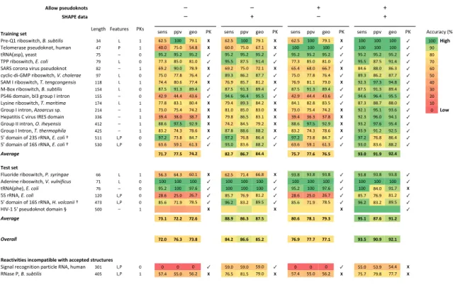
Sensitivities (sens), positive predictive value (ppv), and their geometric average (geo) are shown for four test cases: no pseudoknots allowed and no SHAPE data; no pseudoknots allowed and with SHAPE data (both by free energy minimization); pseudoknots allowed and no SHAPE data; and pseudoknots allowed and with SHAPE data (both using ShapeKnots). Complicating features are ligand (L) and protein (P) binding that are not accounted for in nearest-neighbor thermodynamic parameters. Pseudoknot (PK) predictions are indicated with a checkmark ( ) or X; a checkmark indicates that pseudoknots were predicted correctly and that there were no false-positive pseudoknot predictions. For the ribosomal RNAs (†), regions in which the SHAPE reactivities were clearly incompatible with the accepted structure, as described 18, were omitted from the sensitivity and ppv calculations; for the E. coli 16 rRNA, this included nucleotides 143-220. The HIV-1 5' leader domain (§) was included as an example of pseudoknot prediction in a large RNA. Because the accepted structure for this RNA is based on SHAPE-directed prediction 19, we did not include sensitivity and ppv for this RNA in the overall Average values; however, the pseudoknot was proven independently 20 and is included.

!""#$%&'()*#+,#-' ./!01%*2-2

!"#! $$% &"' () !"#! $$% &"' () !"#! $$% &"' () !"#! $$% &"' () *++,-.+/0123

(-"4560-78'!97:+;<0!"#$%&'()($ => ? 6 @ABC 6DD EFB6 3 @ABC 6DD EFB6 3 @ABC 6DD EFB6 3 6DD 6DD 6DD ✓ 6DD%/456

G"H'I"-.!"0$!",J'K#':<0;,I.# >E ( 6 >DBD ECBD C>BL 3 @DBD ECBD @EB6 3 6DD 6DD 6DD ✓ 6DD 6DD 6DD ✓ FD

:MN*1.!$3<0/".!: EC O D FCBA FCBA FCBA ✓ FCBA FCBA FCBA ✓ FCBA FCBA FCBA ✓ FCBA FCBA FCBA ✓ LD

G((0-78'!97:+;<#*"#+,)( EF ? D EEB= LCBD L6BD ✓ FCBC LEBC F6B> ✓ EEB= LCBD L6BD ✓ FCBC LEBC F6B> ✓ ED

P*MP0+'-'#.0%7-,!0$!",J'K#':0 LA O 6 @FBA FDBD ELBF 3 @FBA ECBD EAB6 3 @CB> @LBD @@BE 3 L>B@ LLBD L@B= ✓ @D

+/+H7+4J74QR(0-78'!97:+;<#-"#+.,)/01/# FE ? D ECBD EEBL E@B> ✓ LFB= L@BA LEBE ✓ ECBD EEBL E@B> ✓ LFB= L@BA LEBE ✓ CD

P*R0S0-78'!97:+;<#2"#'/34+,34/3$($ 66L ? 6 E>B> LDB@ EEB> 3 E@BF LCBE L6BA 3 E@BF L6B6 EFBD 3 FAB= FEB= F>BL ✓ >D

R4T'U0-78'!97:+;<0!"#$%&'()($0 6C> ? D LEBC F6B= LFB> ✓ LEBC F6B= LFB> ✓ LEBC F6B= LFB> ✓ LEBC F6B= LFB> ✓ =D

(C>@0J'I.7#<08S=0&-',$0S07#:-'# 6CC O D >ABF >>B> >=B@ ✓ F>B@ F@B> FCBC ✓ >ABF >>B> >=B@ ✓ F>B@ F@B> FCBC ✓ AD

?/!7#"0-78'!97:+;<02"#510('(51 6E> ? 6 EEBL L=B6 LDB> 3 EFB> LFB= L>BA 3 L>B6 LABL L=BC ✓ LEB= LLBE LLBD ✓ 6D

Q-',$0S07#:-'#<#67,10+%$0!$B A6> O 6 E=BD ECB> E>BA 3 L6BD LCBD L=BD 3 E=BD ECB> E>BA 3 FAB6 FCB6 F=B@ ✓ D %7#$

V"$.:7:7!0W0%7-,!0SMXP0J'I.7# ==@ O 6 =FB> =LBD =LBE 3 EFBL L@BC L=B6 3 =FB> =@B= =EBL 3 FAB= F@BD F>B6 ✓

Q-',$0SS07#:-'#<08"#(./9/3$($# >6A O 6 LLB@ FEBC FABF 3 E>BA L>BC EFBA 3 LLB@ FEBC FABF 3 F=BA FEB@ FCB> ✓

Q-',$0S0S#:-'#<#2"#'./05,:.()1 >AC O 6 L=BA E>B= ELB@ 3 LEBL LLB@ LLBA 3 L=BA E>B= ELB@ 3 F=BF F6BA FABC ✓

CY0J'I.7#0'Z0A=P0-MN*<0*"#+,)(0[ C66 ?<( D FEBA E=BL L>BE ✓ FEBA E@BL L@B> ✓ FEBA E=BL L>BE ✓ FEBA E@BL L@B> ✓

CY0J'I.7#0'Z06@P0-MN*<#*"#+,)(0[ C=D ?<( D @=B@ CFB6 @6B= ✓ F=BD L=B@ LLBA ✓ @=B@ CFB6 @6B= ✓ F=BD L=B@ LLBA ✓

!"#$%&# 89:8 88:; 8<:= >=:8 >?:8 ><:< 8;:8 88:? 8?:; @A:B @9:@ @=:<

C('-%'(-\H,'-7J"0-78'!97:+;<#;"#$90(341/ @@ ? 6 C@B= @>B= @DB6 3 @ABC E6B> @@BL 3 F=BL F=BL F=BL ✓ F=BL F=BL F=BL ✓

*J"#7#"0-78'!97:+;<0-"#<%)3(=(+%$ E6 ? D 6DD 6DD 6DD ✓ 6DD 6DD 6DD ✓ 6DD 6DD 6DD ✓ 6DD 6DD 6DD ✓

:MN*1$;"3<#*"#+,)( E@ O D FCBA 6DD FEB@ ✓ 6DD 6DD 6DD ✓ FCBA 6DD FEB@ ✓ 6DD L>BD F6BE 3

CP0-MN*<0*"#+,)( 6AD ?<( D ALB@ ACBD A@BE ✓ LCBE E@BF L6BA ✓ ALB@ ACBD A@BE ✓ LCBE E@BF L6BA ✓

CY0J'I.7#0'Z06@P0-MN*<0>"#<,)+13((0[ >E= ?<( D LCB@ E6BF ELBC ✓ F@BA L=BA LFBC ✓ LCB@ E6BF ELBC ✓ F@BA L=BA LFBC ✓

VS]460CY0$!",J'K#':0J'I.7#0^ CDD O 6 >@BL =CBL

>DBF 3

EEBC LLBD

LAB@ 3

LDBD LDBD

LDBD 3

6DD 6DD

6DDBD ✓

!"#$%&# 8A:9 8=:= 8=:? >>:@ >?:A >8:; >B:? 8>:9 8@:A @;:9 >8:? @9:=

'"#$%(( 8=:B 8?:A 8A:> ><:= >?:? >;:= 8?:@ 88:8 88:9 @A:; @B:@ @=:9

D(2E-4F4-4('%4,E#G&2-4H"(%$4-6%2EE(&-(*%'-I)E-)I('

P7&#.H0-"+'&#7:7'#0$.-:7+H"0MN*<0;,I.# =D6 ?<( D D D D ✓ CFBD CFBD CFBD ✓ D D D ✓ CCBD C=BF C>B> 3

MN.!"0(<0!"#$%&'()($# >DC ?<( 6 CEB> CCBD C@BA 3 E@BC L6BC EFBD 3 CEB> CCBD C@BA 3 ECBE EFBL EEBE 3

Hajdin et al., Table 1

CI24,4,5%'(- ?"#&:; \".:,-"! ()!

O O _ _

(33)

The structures of the 16 RNAs in the test set are predicted poorly by a conventional algorithm based on their sequences alone: The average sensitivity (sens; fraction of base pairs in the accepted structure predicted correctly), positive predictive value (ppv, the fraction of predicted pairs that occur in the accepted structure), and geometric average of these metrics are 72, 78, and 74%, respectively (Table 2.1).

In the process of developing this training set, we also analyzed two RNAs – RNase P RNA and the human signal recognition particle RNA – whose in vitro SHAPE reactivities were incompatible with the accepted structures for these RNAs. I include prediction statistics for these RNAs at the bottom of Table 2.1, but do not use these to evaluate our SHAPE-directed modeling algorithm.

2.2.2A simple, robust model for pseudoknot formation.

The favorable energetic contributions for forming the helices that comprise a pseudoknot are likely to be predicted accurately by the Turner nearest-neighbor model 17, 21 _{when modified by the experimental}_∆_G_{°SHAPE term (Eqn. 1). In addition, pseudoknot}

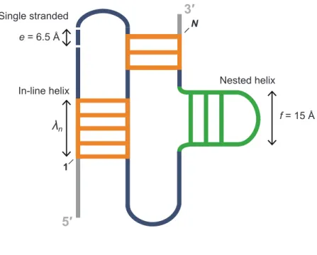
formation must overcome an entropic penalty; these energetics are difficult to estimate. The most widely used models are complex and include a large number of constituent parameters11, 12_{. We adopted a simple approach to estimate the entropies based on three}

(34)

We modeled RNA pseudoknots as the sum of simple distance features, or beads. There are exactly three possibilities for the structures that comprise a pseudoknot: single-stranded nucleotides, nested helices, and in-line helices (Figure 2.1). Duplexes containing single nucleotide bulges are counted as a single helix. This model emphasizes structures rather than topologies and appears to be compatible with the vast majority of known pseudoknots. In essence, energetically favorable pseudoknots feature a small number of the single-stranded, nested helix, and in-line helix “beads.” To account for the number of constituent single-stranded (SS) nucleotides and nested (NE) helices (Figure 2.1), we adopted a simple polymer physics-based model 22. The energetic penalty associated with each of these features is weighted by distances of e = 6.5 Å and f = 15 Å, the mean lengths of a single-stranded nucleotide and a nested helix element, respectively22_(Figure

1). Finally, we created a penalty for in-line (IL) helices (Figure 2.1). The potential to form these structures is weighted by their end-to-end length (n) in the context of A-form helix geometry and the distribution of in-line helices in RNAs of known structure. The model for the entropic cost of pseudoknot formation, ∆G°PK, has two adjustable parameters, P1 and P2:

∆G°PK = P1ln (e2SS + f 2NE) + P2lnΣIL(n)(λn2) (2)

where λn is the penalty constant for in-line helices of length n (see Table 2.2). The first

(35)

Figure 2.1: Overview of pseudoknot structure model and entropic penalty terms.

Length features are incorporated into ∆G°PK as described in Eqn. 2. Energy penalties for single-stranded nucleotides and nested helices are based on a previously developed model 22_{; the penalty for in-line helices was developed in this work.}

5

3

Single'stranded

e'='6.5'Å

Nested'helix In6line'helix

f'='15'Å

1

N

Hajdin'et'al.,'Figure'1

(36)

____

Helix Length (n) pn (Å) qn λn = pn / qn

_________________________________________________________________________

2 0 0.0000 0

3 6.1 0.2546 24

4 11.9 0.4975 24

5 16.9 0.4962 34

6 20.9 0.8795 24

7 23.8 0.6869 35

8 25.5 0.4430 58

9 26.4 0.3217 82

10 26.8 0.4104 65

11 27.4 0.0519 527

12 28.6 0.0117 2447

13 30.9 0.0074 4199

14 34.1 0.0052 6564

15 38.0 0.0030 12540

_________________________________________________________________________

Table 2.2:Energy penalty per in-line pseudoknotted helix of length n.

pn is the end-to-end distance (in Å) between the C4' of the first and last nucleotide of an

(in-line) helix of length n. The value qn was calculated in two steps. First, for five classes

of RNA – group I introns 24, 25, RNase P 26, SRP 27, tmRNA 28 and telomerase29 – we calculated the fraction of in-line helices of length n over the total number of pseudoknotted structures in each class of RNA. Second, we averaged the fractions of length n across the five RNA classes. λn, the penalty constant for an in-line helix of

(37)

2.2.3RNA structure interrogation by SHAPE.

Most RNAs were transcribed in vitro and contained short hairpin-containing structure cassettes at their 5’ and 3’ ends 23. The 16S and 23S ribosomal RNAs were isolated from total E. coli RNA15_{. The transcribed RNAs were folded in a standard buffer}

with physiologically relevant ion concentrations (and saturating ligand concentrations for riboswitches) and treated with 1-methyl-7-nitroisatoic anhydride (1M7)30_{. Sites of 2'-}_O

-adduct formation were detected by primer extension using a previously described high-throughput SHAPE approach31

. SHAPE reactivities were normalized to place them on a

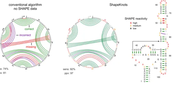
scale from zero (unreactive) to ~1.5 (highly reactive). In this work, we illustrate modeling results in the form of circle plots, which provide an unbiased way to visualize correct and incorrect base pairs. The nucleotide sequence is arrayed on the outer circle: unreactive nucleotides (SHAPE reactivities < 0.4) are colored black, moderately reactive nucleotides (0.4 – 0.85) are yellow, and highly reactive nucleotides (> 0.85) are red. Base pairs are shown as arcs, colored by whether they are predicted correctly or not (Figure 2.2). Pseudoknots correspond to helices whose arcs cross in the circle plot. In general, there was a strong correspondence between SHAPE reactivities and the pattern of base pairing in the accepted structures. Nucleotides that participate in canonical base pairs were generally unreactive; whereas nucleotides in loops, bulges, and other connecting regions were reactive (Figure 2.2).

2.2.4Algorithm and Parameter Determination.

(38)

Figure 2.2: Representative ShapeKnots structure prediction for the SAM I riboswitch.

In all panels, base pair predictions are illustrated with colored lines: green, correctly predicted; red, missed base pair relative to the accepted 32_{structure; purple, prediction of} a pair not in the accepted structure. Left-hand panel shows predictions without SHAPE data. Center and right-hand panels show predictions made when SHAPE data were included, using circle plot and conventional representations, respectively. Sensitivity (sens) and ppv are listed for each structure. SHAPE data are shown as colored nucleotide letters on a black, yellow, red scale for low, medium and high SHAPE reactivities, respectively.

U 1

U C U U A UCAA10_{G A}

G A_A

G_C A_G

A 20_G G G_A C U G G C C 30 C G A C G A A G C U 40 U C A G C A A CC G 50 GU G UA AU GG C 60 GA UC A G CC A U 70 GA C C A A G G U G80 C U A A A U C C A G 90C A AG CU CG AA

100CA

GC

UU

GGA A 110GA UAA G A

A 118 conventional*algorithm no*SHAPE*data ShapeKnots* 10 A G C A U 4 U A U A C G U A U A A U U A C G A A G A U 0 G C C G

A GA

20 G C G C 30 G C

A CU GA 90 G C G C G A C G A A A U G C C G 80

A

AC G

C G

G 50 G CC

U A

G

UA

A U 70 U A G C GC C 60 G G

A U C A G A A U A A A U C G A U A U G C C G U A C G A A 100 C G A A 110 missing

U1_{U C U U A U} C AA10_{G A}

G A A_G C A_G A 20 G_G G A C U G G C C 30 C G A C G A A G C U 40 U C A G C A A C C G₅₀ GU GU AA UG G C 60 GA UC AG CC A U 70 GA C C A A G G U G80 C U A A A U C C A G 90C A A GC UC GA A 100CA

GC

UUG

G AA

110G AU A

A G AA

(39)

and low SHAPE reactivities, respectively, are universal to all RNAs, and do not directly contribute to the entropic penalty for pseudoknot formation. These parameters can thus be fit independently of the ΔG°PK terms, P1 and P2. m and b were optimized using the seven RNAs in our dataset that do not contain pseudoknots. To reduce over-optimization of these parameters, we used a leave-one-out jackknife approach33_{to assess prediction}

sensitivities, ppv, and the geometric mean of these parameters at each grid point for seven quasi-independent data sets each containing six of the seven RNAs.

Our algorithm for identification of pseudoknots follows the approach implemented in HotKnots10

. A two-stage refinement first finds stable helices using a

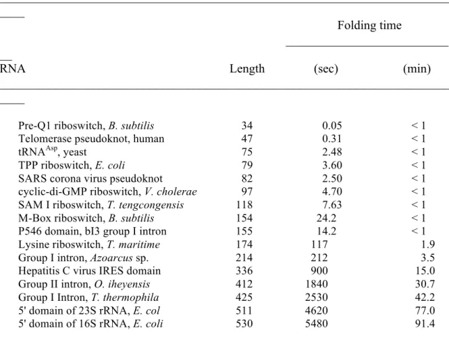
dynamic programming algorithm that does not allow pseudoknots. The second stage uses the same dynamic programming algorithm to predict structures for each stable helix found in stage one. In stage two, structures are predicted such that nucleotides in the stable helix are forced to not pair. These pairs are subsequently added back to the structure, and these helices can therefore be pseudoknotted. This allows the prediction of up to one pseudoknot per run. Run times for the final ShapeKnots algorithm were less than 1 min for RNAs of fewer than 150 nts and ~90 min for the longest (530 nt) RNA (Table 2.3).

(40)

Figure 2.3: Optimization of the ∆G°SHAPE and ∆G°PK parameters (in kcal/mol) by jackknifing.

Each of the three panels shows a representative grid in which the M-box RNA was left out. Optimal parameters in each case are emphasized with a white box. Each box in the grid represents the accuracy (calculated as the geometric mean of sens and ppv) for the test set at each slope and intercept for Steps 1 and 3, and each P1 and P2 value for Step 2. For clarity, only a subset of parameter optimizations is shown.

0.15 0.25 0.35 0.45 0.55

0.25 85.8 85.8 85.8 85.8 85.8 85.8 85.8 85.8 85.8

85.8 85.8 85.8 85.8 85.8 85.8 85.8 86.0 86.5

0.35 85.8 85.8 85.8 85.8 85.8 86.0 86.0 86.5 86.5

85.7 85.7 85.7 85.9 85.9 85.9 86.4 86.5 89.9

0.45 85.7 85.8 86.0 85.8 86.5 86.3 89.6 89.6 91.2

85.8 85.8 85.8 86.3 86.3 89.4 89.6 91.0 88.8

0.55 86.5 85.8 87.0 86.3 90.1 89.6 91.7 88.8 88.5

85.8 86.3 86.3 89.4 89.6 91.0 88.8 88.3 88.3

0.65 87.0 86.3 90.1 89.6 91.7 88.1 88.5 88.3 88.5

86.3 89.4 89.6 91.0 88.1 88.3 88.3 88.3 88.3

0.75 90.1 91.0 91.7 88.1 88.5 88.3 88.5 88.3 88.5

91.0 90.2 88.1 88.3 88.3 88.3 88.3 87.4 87.4

0.85 90.9 88.3 88.5 88.3 88.5 88.3 87.6 86.3 86.5

88.3 88.3 88.3 88.3 87.2 86.3 86.3 86.3 86.3

0.95 88.5 88.3 87.4 87.2 86.5 86.3 86.5 86.3 86.5

87.2 87.2 87.2 86.3 86.3 86.3 86.3 86.3 86.2

1.05 87.4 87.2 86.5 86.3 86.5 86.3 86.4 86.2 86.4

86.3 86.3 86.3 86.3 86.2 86.2 86.2 86.2 86.2

1.15 86.5 86.2 86.4 86.2 86.4 86.2 86.4 86.2 86.4

Step01:0Optimize0Slope0and0Intercept0

0 0over070non?pseudoknotted0RNAs

Accuracy

low high Step02:0Optimize0P10and0P20over0160RNAs

Step03:0Optimize0Slope0and0Intercept0over0160RNAs

Hajdin0et0al.,0Figure0S1 P1

P2

Intercept

Slope Slope

Intercept

1.4 1.6 1.8 2.0 2.2 2.4 2.6 2.8 3.0 3.2 3.4 3.6 3.8 4.0

0.0 79.1 78.8 79.0 75.0 74.5 73.5 73.6 73.5 73.2 73.2 73.2 73.0 73.0 72.9 72.6 72.5 72.1 71.6 71.5 71.5 71.0 69.9 69.4 69.9 69.8 69.8 69.7 78.7 78.7 79.1 79.7 79.7 78.5 78.5 77.6 77.5 77.6 77.6 73.7 73.7 73.6 73.2 72.8 72.9 72.9 72.9 72.8 72.6 72.1 72.0 72.1 71.5 71.4 71.3 ?0.2 81.2 80.9 81.1 81.1 81.0 80.9 81.6 81.6 81.4 81.4 80.5 78.6 78.4 77.6 77.3 76.9 77.1 76.9 77.3 75.5 75.5 75.3 75.2 75.3 75.0 75.0 74.5 84.2 84.0 84.0 82.1 80.2 81.0 81.0 81.3 81.4 81.4 81.4 81.4 80.4 80.2 80.2 80.1 80.3 80.2 80.1 79.9 79.9 79.6 78.8 78.8 76.5 76.3 74.2 ?0.4 87.5 86.5 86.5 86.3 84.2 84.1 84.0 83.6 81.6 80.6 81.4 81.4 83.3 81.4 80.4 82.8 82.8 82.8 84.0 83.0 81.7 81.6 82.5 82.5 82.3 81.4 82.0 90.5 89.3 89.4 89.4 89.7 89.7 89.5 87.1 86.2 85.9 85.6 85.4 80.3 83.7 81.0 81.6 84.9 83.9 84.9 85.6 85.6 85.6 83.8 82.5 82.6 82.5 82.5

?0.6 90.1 89.1 89.289.289.2 89.7 89.7 89.7 89.7 89.4 87.3 87.2 86.0 85.6 85.4 85.5 85.5 83.9 81.3 84.9 84.0 84.0 84.8 84.8 83.5 83.5 81.3

83.7 88.6 88.4 88.9 89.1 89.1 89.5 89.2 89.5 89.5 89.8 89.6 90.0 89.7 87.9 86.7 85.5 85.5 86.3 86.3 81.3 81.3 83.6 82.3 82.7 82.6 82.6

?0.8 83.3 87.6 88.1 82.2 89.1 88.6 89.2 89.0 89.4 89.4 89.5 90.0 90.090.091.0 90.7 89.8 89.6 87.9 86.4 86.3 86.4 86.3 85.6 84.3 84.3 84.1

83.6 81.3 88.1 82.2 81.9 88.5 88.5 88.6 89.0 89.1 89.2 89.3 89.4 89.3 90.7 90.6 89.9 90.2 90.7 90.5 90.5 87.9 86.5 85.8 85.6 85.6 85.0 ?1.0 79.3 82.1 81.6 81.8 81.9 88.5 88.5 82.4 89.0 89.0 89.0 89.0 89.2 89.2 90.0 90.1 89.9 89.8 90.9 90.9 90.9 90.5 90.5 90.8 88.3 86.8 86.8

78.9 77.8 82.1 82.1 81.5 82.0 82.0 82.2 88.5 88.9 89.1 89.0 89.0 89.0 89.9 90.0 89.2 89.3 90.1 90.0 90.9 90.9 90.991.291.0 90.8 90.6

?1.2 76.6 78.0 77.7 77.3 82.0 82.0 82.0 82.0 82.0 82.0 82.6 82.6 82.7 89.2 89.8 89.8 89.1 89.2 90.1 90.1 90.1 89.9 90.5 91.2 91.2 91.2 91.1 76.6 76.9 77.7 77.7 77.0 81.7 82.0 82.0 82.0 82.0 82.0 82.4 82.6 82.8 90.0 90.0 89.2 89.2 89.9 89.9 90.1 90.1 90.1 90.4 90.3 90.6 91.2 ?1.4 76.3 76.9 76.6 76.6 76.9 76.9 80.5 82.1 82.0 80.9 80.9 81.3 82.4 82.4 82.4 82.8 82.8 82.8 90.0 89.9 90.1 90.0 90.0 90.4 90.4 90.4 90.2 76.2 76.6 76.8 76.6 76.9 76.9 76.9 76.8 80.9 80.8 80.8 80.8 82.4 82.4 82.4 82.4 82.4 82.8 90.0 90.0 90.0 90.0 90.1 90.4 90.4 90.3 90.3 ?1.6 76.4 76.5 76.6 76.8 76.9 77.1 76.9 76.5 76.4 80.5 80.8 80.8 80.9 80.9 81.3 82.4 82.4 82.4 82.4 82.7 82.8 82.8 90.0 90.4 90.4 90.3 90.4 71.9 73.6 76.2 76.6 76.9 76.9 77.1 76.5 76.5 76.5 80.4 80.5 80.8 80.8 81.5 81.5 81.5 82.7 82.7 82.7 82.4 82.6 82.8 83.1 90.4 90.4 90.4 ?1.8 71.1 72.8 71.1 72.7 73.3 76.9 76.9 76.3 73.0 76.5 76.5 75.8 80.5 80.8 81.4 81.4 81.5 81.5 81.5 81.5 81.5 81.5 82.7 81.7 83.1 83.1 83.1 70 71.4 71.1 72.5 71.2 73.0 73.0 73.3 72.7 72.7 73.0 75.8 72.7 79.7 81.1 81.1 81.4 81.5 81.5 81.5 81.5 81.5 81.5 81.5 81.6 81.7 81.8 ?2.0 67.5 67.8 71.1 71.1 71.4 71.2 73.0 73.3 71.3 72.7 72.7 72.7 72.7 72.7 72.7 76.5 81.1 81.1 81.4 81.5 81.5 81.5 81.5 81.5 81.5 81.5 81.6 67.6 67.8 67.5 67.5 68.9 71.4 71.2 73.3 71.3 71.3 72.7 72.7 72.7 72.7 72.7 72.7 76.5 76.9 78.0 81.4 81.5 81.5 81.5 81.5 81.5 81.5 81.5 ?2.2 67.6 67.6 67.5 67.5 67.8 68.2 68.9 71.5 71.3 71.3 71.3 72.7 72.7 72.7 72.7 72.7 72.7 76.5 76.5 76.9 78.1 78.5 78.5 78.4 81.5 81.5 81.5 55.1 67.6 67.6 67.6 67.8 67.8 68.2 68.2 68.6 68.8 71.3 72.7 72.7 72.7 72.7 72.7 72.7 72.7 76.6 76.5 76.7 78.1 78.1 78.5 78.5 78.4 78.4

1.4 1.6 1.8 2.0 2.2 2.4 2.6 2.8 3.0 3.2 3.4 3.6 3.8 4.0

(41)

Table 2.3:ShapeKnots run times as a function of RNA length.

________________________________________________________________________ ____

Folding time

__________________________ __

RNA Length (sec) (min)

________________________________________________________________________ ____

Pre-Q1 riboswitch, B. subtilis 34 0.05 < 1

Telomerase pseudoknot, human 47 0.31 < 1

tRNAAsp_{, yeast} ₇₅ _2.48 _{< 1}

TPP riboswitch, E. coli 79 3.60 < 1

SARS corona virus pseudoknot 82 2.50 < 1

cyclic-di-GMP riboswitch, V. cholerae 97 4.70 < 1

SAM I riboswitch, T. tengcongensis 118 7.63 < 1

M-Box riboswitch, B. subtilis 154 24.2 < 1

P546 domain, bI3 group I intron 155 14.2 < 1

Lysine riboswitch, T. maritime 174 117 1.9

Group I intron, Azoarcus sp. 214 212 3.5

Hepatitis C virus IRES domain 336 900 15.0

Group II intron, O. iheyensis 412 1840 30.7

Group I Intron, T. thermophila 425 2530 42.2

5' domain of 23S rRNA, E. col 511 4620 77.0

5' domain of 16S rRNA, E. coli 530 5480 91.4

________________________________________________________________________ ____

(42)

We recommend use of these new values for RNA structure prediction both with and without pseudoknots. Applying ShapeKnots using these ∆G°SHAPE and ∆G°PK parameters yielded an average sensitivity for secondary structure prediction of 93% for the sixteen RNAs in the test set (Table 2.1).

2.2.5Extension to additional RNAs.

We used ShapeKnots to model secondary structures for six RNAs that were not used to optimize the final algorithm. Three RNAs – the adenine riboswitch, tRNAPhe,

and E. coli 5S rRNA – were chosen because prior approaches using non-standard data

analysis had suggested that they folded poorly with SHAPE data16

. The other three RNAs

– the fluoride riboswitch pseudoknot, 5' domain of the H. volcanii 16S rRNA, and the 5' pseudoknot leader of the HIV-1 RNA genome – adopt structures that are predicted poorly by conventional approaches. Overall prediction sensitivities for these six RNAs were ~95% (Table 1), and the pseudoknots in the HIV-1 and fluoride riboswitch RNAs 34-36

were identified correctly

2.3Discussion

Pseudoknots are relatively rare in large RNAs but are highly overrepresented in important functional regions2, 3, 6, 7_._{Despite their importance, the most commonly used}

(43)

(44)

Table 2.4:Prediction accuracies for seven RNA folding algorithms (following page). A) Overall prediction accuracies. Accuracies are shown as percent sensitivity (sens) and positive predictive value (ppv), and allow pairing to be shifted by one position on one side of a pair 37. ShapeKnots, ProbKnot 13, and Fold (the standard RNAstructure algorithm) 38 were run both with and without SHAPE data. Other included algorithms are DotKnot+KL and DotKnot-KL (KL indicates kissing loops) 39, 40, ipknot 41, pknotsRG-mfe 42, and HotKnots 12. Note that Fold does not allow pseudoknots. All algorithms were run using their default parameters. ShapeKnots, Fold and ProbKnot used

m and b parameters (Eqn. 1) of 1.8 and -0.6 kcal/mol, respectively.

B) Prediction accuracies for pseudoknotted base pairs only. Accuracies are evaluated using sensitivity and ppv, allowing for mis-pairing by one position on one side of a pair 37_{. If both accepted and predicted structures contain no pseudoknot, sens and ppv are} defined as 100%. If only the predicted structure contains a pseudoknot, sens and ppv are set to 0. A pseudoknotted pair is scored as correctly predicted only if there is at least one other correctly predicted pair with which it forms a pseudoknot. Fold is excluded because it does not allow prediction of pseudoknots.

(45)

The prediction sensitivity for base pairs that specifically form pseudoknots varies by algorithm and benchmark RNAs but averages only 5-20%, with many false-positive predictions13 (Table 2.4). Thus, the current generation of pseudoknot prediction algorithms is poorly suited for designing testable biological hypotheses.

ShapeKnots combines an iterative pseudoknot discovery algorithm with experimental SHAPE information and a simple energy model for the entropic cost of pseudoknot formation. The pseudoknot penalty in ShapeKnots has only two adjustable parameters (Figure 2.1 and Eqn. 2) that limit formation of pseudoknots with long single-stranded regions and many nested helices and that enforce an optimal geometry for in-line helices. ShapeKnots also allows incorporation of an experimental correction to standard free energy terms. Including SHAPE data both limits the number of possible structures and provides information that accounts for hidden features that stabilize RNA folding, including the significant effects of metal ion and ligand binding.

(46)

We summarize our modeling results by emphasizing four classes of RNA: (i) short pseudoknotted RNAs with structures that ShapeKnots predicts very accurately, (ii) large, challenging RNAs that ShapeKnots predicts with good accuracy, (iii) RNAs with high likelihood of being mischaracterized with false-positive or missed pseudoknots that ShapeKnots predicts accurately, and (iv) RNAs that interact with other molecules such as ligands, proteins, and metal ions that pose unique challenges. For most RNAs analyzed here, differences between models generated by ShapeKnots and currently accepted structures were minor and typically involved short-range interactions or base pairs at the ends of helices. In some cases, differences likely reflect thermodynamically accessible states at equilibrium in solution.

2.3.2Short pseudoknotted RNAs.

The first class includes small RNAs that contain H-type pseudoknots: the pre-Q1 riboswitch, human telomerase, the fluoride riboswitch, and a SARS corona virus domain. Because the most commonly used dynamic programming algorithms cannot predict base pairs in an H-type pseudoknot, prediction sensitivities using a conventional algorithm38 were quite poor; in contrast, ShapeKnots yielded perfect or near-perfect predictions in each case (Figure 2.4). The only ShapeKnots-predicted base pairs that do not occur in the accepted structures involve sets of two or fewer base pairs located at the ends of individual helices in the fluoride riboswitch and SARS domain. These results suggest that ShapeKnots prediction of H-type pseudoknots in short RNAs is robust.

(47)

Figure 2.4: Summary of predictions for four H-type pseudoknots.

Base pair predictions are illustrated as outlined in Figure 2.2; sensitivity (sens) and ppv are listed for each structure. Left- and right-hand columns show predictions for a conventional mfold-class algorithm versus ShapeKnots (with experimental SHAPE restraints).

G 1

C AU_{U G}

G A_G

A 10_U

G G C A U U C C U 20 C C A U U A A C A A 30 AC CG CU GC G C 40 C C G U A G C A G C 50U GA UG AU GC C 60U AC

A GA

66 Pre$Q1'riboswitch

Telomerase

SARS'virus'domain

conventional,'no'data ShapeKnots

A1G A_G

G U U C U A 10 G C U A CA CC CU 20 CU A U A A AA AA

30 CU

A A

34

Hajdin'et'al.,'Figure'3 A1G A_G

G_U U C U A 10 G C U A CA CC C U 20 C U A U A A A AA A

30CU

AA

34

G 1

G G CU

G U U U U 10 U C U C G C U G A C 20U UU CA GC CC A 30 A C A C A A AA AA 40 A GU

CA G

C 47

G1_{G G C}

U G_U

U U U 10 U C U C G C U G A C 20 UU UC AG C CC A 30 A C A C A A AA AA 40A GU

C AG

C 47

U1_{U U A A}

A C_{G G}

G10_U

U U G C G G U G U 20 A A G U G C A G C C 30C G U CU UA CA C 40 CG UG CG GC AC 50 A G G C A C U A G U 60A C U GA UG UC G 70 UC

UA

CA

G GG C

U U82 U1UUA_{A A}

C G

G_G10

U U U G C G G U G U 20 A A G U G C A G C C 30 C G U C UU AC AC 40 C G UG CG GC AC 50 A G G C A C U A G U 60 A C U G AU GU CG

70UC

UA

CAG G

GC U U

82

G1_{C A U U}

G G A_G A 10 U G G C A U U C C U 20 C C A U U A A CA A 30 AC CG CU GC G C 40 C C G U A G C A G C 50U GA UG AU GC C

60U AC A

(48)

2.3.1Large, complex RNAs.

The second class includes large RNAs that do not require ligands or protein co-factors for correct folding. Large RNAs pose a challenge to modeling algorithms due to the vast number of possible structures and due to the large number of structures with similar folding free energies changes. For example, in the absence of experimental structure probing data, two representative RNAs, the Azoarcus group I intron and the hepatitis C virus IRES domain are predicted with sensitivities of 73 and 39%, respectively. Mis-predictions occur primarily in two hairpin motifs in the Azoarcus RNA but span essentially the entire HCV IRES RNA (Figure 2.5). Inclusion of SHAPE data yielded near-perfect predictions in each case, including correct identification of the pseudoknot in each RNA (Figure 2.5).

2.3.2RNAs with difficult to predict pseudoknots.

(49)

Figure 2.5: Prediction summaries for two large, pseudoknot-containing RNAs.

Structural annotations are as described in Figure 2.2.

C 1

U C A U A UU UC10G AUGU_{G C} C UU20_{G C}

GCCGGGA

A 30A

CC AC G C AA G 40 G G A U G G U G U C 50 A A A U U C G G C G 60 A A A C C U A A G C 70 G C C C G C C C G G 80 G C G UA U GG C A_90AC GC CG AG C C 10 0AA GC UU CG G C 11 0G CC UG C GC C G 12 0AU GA A GG UG U 13

0GA

A G A C U A GA14

0GC

G C A C C C A C 150C U A A G G C A A A 160C G CU A U GG UG

170AA

GG

CA UA

GU

180CC

AGG

GA

GUG

190GCGAA AG U

C200ACA CAA A

CC G210GAA UC214

conventional,+no+data ShapeKnots

Hajdin+et+al.,+Figure+4 C

1

CA UGAA UCA10CUCCCCU_GUG20A

GGA_ACUAC U30 GUCU UCAC GC40 AG AAAG CG UC 50UAGCC

AUGGC 60GU

UAGUAUGA 70GUGU

CG

U

G

CA 80GCCU

C

A

G

A 90

C C C C C C C U C C 100C G G G A G A G C C 110A U A G U G G U C U120G C GG A A CC GG 13 0 UG AG UA CA CC 140 GGA AU UG CC A 150 GG AC GA CC GG 16 0GU CC UU UC UU 170 GG AU UA AC CC 18 0GC UC AA UG CC1 90 UG GA GA UU UG 20 0GG CG UG CC CC 21 0CG CG A G A CU G220 C UA G C C GA GU230 A G U G U U G G G U

240CG

C G AA A G G C 2

50 CUUGUG

G

U

A

C

26

0UGCC

U

GAUAG 270 GG

UGCUUGC280 AGGUGCCCCG29G0GAG GUCU

CGU30 0 AGAC

CGUG C A310UC

A UGAGCAC320GA AUCCUA A A330CCU CA A 336

Hepatitis+C+virus+IRES+domain+(336+nts)

Azoarcus+group+I+intron+(214+nts)

sens:+73% ppv:+75

C1_{U C A U A U U U}

C10_{G A U}

G U G_{C C}

UU20_{G C}

GCCGG

GAA 30 AC CA C GC A A G 40 G G A U G G U G U C 50 A A A U U C G G C G 60 A A A C C U A A G C 70 G C C C G C C C G G80 G C G UA UG GC A 90 AC GC CG AG C C 10 0AA GC UU CG G C 11 0GC CU GC GC C G 12 0AU GA AG GU G U 13 0AG A G A C U A G A14

0GC

G C A C C C A C 150C U A A G G C A A A 160C G C U A UG GU G

170AA GG

CA

UA

GU 180CCA

GGG AG

UG 190GCG AA A

G UC A 200C AC A

A A CC GG

210

A A UC214

C 1

CA U G A AUCA10CU CCC C UGUG20

A G GAA CU ACU30

G UC UUCA C

GC40AG AA

AG CGU

C 50UA

GCC

AUGGC 60GUU A GUAUG

A 70

G

U

GUCGUGCA 8GC0

CUCCA

G

A 90

C C C C C C C U C C 100 C GG G A G A G C C 110 A U A G UG G U C U120 G C G G A A C C G G 13 0 U GA GU A CA C C 140 GG AA UUG CC A 150 GG AC GA CC G G 16 0GU CC U UU CU U 170 GG A UU A ACC C 18 0G CU C AA UG C C19 0UG G AG A UU U G 20 0GG C G UG C C C C 21

0GC

C G A G A C U G220 C U A G C C G A G U 230A G U G U U G GG U 240C G C G A A A G G C 25

0CUUGUGGU

A

C

2

60UGCCUGAUA

G

270GGUGCUUG

CG

280AGUGCCCC29GG0GAGGUCU

CG30U0AG AC C

(50)

Figure 2.6: Representative examples in which ShapeKnots avoids false-positive (top) or false-negative (bottom) pseudoknot predictions.

Left- and right-hand panels show the results of ShapeKnots predictions without and with SHAPE data, respectively. The bold arrow in the left-hand panels emphasizes the

U1_{U C U U A U}

CAA10

G A_{G A}

A G C A_G A 20 G G G A C U G G C C 30 C G A C G A A G C U 40 U C A G C A A CC G 50 GU G UA AU GG C 60 GA UC AG CC A U 70 GA C C A A G G U G80 C U A A A U C C A G 90C A AG CU CG AA

100CA

GC

UU

GGA

A

110GA U

AA G AA

118

U1_{U C U U A U}

C AA10_{G A}

G A_A

G C A G A 20 G G G A C U G G C C 30 C G A C G A A G C U 40 U C A G C A A CC G 50 GU GU AA UG G C 60 GA UC AG CC A U 70 GA C C A A G G U G80 C U A A A U C C A G 90C A AG CU CG AA

100CA

GC

UU

GGA

A

110G AU A

A G AA

118 SAM$I$riboswitch

U1_{U U A A} A C

G G_G10

U U U G C G G U G U 20 A A G U G C A G C C 30 C G U CU UA CA C 40 CG UG CG GC A C 50 A G G C A C U A G U 60 A C U GA UG UC G

70UC

UA

CA G

G GC

80

UU82 U1UUA_{A A}

C G_G

G10 U U U G C G G U G U 20 A A G U G C A G C C 30 C G U C UU AC AC 40 C G UG CG GC AC 50 A G G C A C U A G U 60 A C U GA UG UC G

70 UC

UA

CA

G GG

C U U

82 SARS$corona$virus sens:$65% ppv:$68 sens:$92% ppv:$97 sens:$77% ppv:$81 sens:$85% ppv:$88 Hajdin$et$al.,$Figure$5

5098.pdf

TABLE OF CONTENTS

List of Tables

List of Figures

List of Abbreviations

1.

Chapter 1: Introduction

Simple H-type pseudoknot

Pseudoknot

C

1

C C

U

C

C

C

G

G

U 10

U

G

C

G

AG

UC

C

G

20

GG

A

G

G

U

C

U

C

G

30

U

A

G

A

2.

Chapter 2: ShapeKnots: accurate RNA secondary structure

predictions, including pseudoknots

_{C C}