Particle Path Through a Nested Mach-Zehnder Interferometer

(1)

arXiv:1604.04596v2 [quant-ph] 17 Aug 2016

Particle Path Through a Nested Mach-Zehnder Interferometer

Robert B. Griffiths

∗

Department of Physics

Carnegie Mellon University

Pittsburgh, PA 15213

Version of 1 July 2016

Abstract

Possible paths of a photon passing through a nested Mach-Zehnder interferometer on its way to a detector are analyzed using the consistent histories formulation of quantum mechanics, and confirmed using a set of weak measurements (but not weak values). The results disagree with an analysis by Vaidman [ Phys. Rev. A 87 (2013) 052104 ], and agree with a conclusion reached by Li et al. [ Phys. Rev. A 88 (2013) 046102 ]. However, the analysis casts serious doubt on the claim of Salih et al. (whose authorship includes Li et al.) [ Phys. Rev. Lett. 110 (2013) 170502 ] to have constructed a protocol for counterfactual communication: a channel which can transmit information even though it contains a negligible number of photons.

1 Introduction

This article addresses the question of what one can say about the path of a photon, hereafter called a “particle”, as it passes through the nested Mach-Zehnder interferometer (MZI) shown in Fig. 1 on its way to one of the three detectors. This setup is of interest in and of itself because it raises a question that cannot be answered by standard quantum mechanics as found in standard textbooks: what is a microscopic quantum system actually doing prior to measurement by a macroscopic apparatus? Research in quantum foundations has yet to supply any widely accepted answer to the infamousmeasurement problem: provide a consistent, fully quantum mechanical description of the entire process that goes on in an actual physical measurement of a microscopic system. Indeed, even thefirst measurement problem, understanding how such a measurement can have a well-defined outcome or pointer position, to use the archaic but picturesque language of quantum foundations, rather than a quantum superposition of different and macroscopically distinct positions, has given rise to a long and inconclusive discussion. The failure to settle this first problem has diverted attention from the equally important second measurement problem [1]: how to infer (or retrodict) the earlier micro-scopic property, the one the apparatus was designed to measure, from the final pointer position. Physicists who do experiments frequently interpret the outcomes using realistic language such as: “the detector was triggered by a fast muon traveling from the region where the protons collided.” If quantum theory cannot, at least in principle, make sense of language of this sort, how can one claim that experiment has confirmed what is often said to be a very successful physical theory?

In addition to its intrinsic interest, the gedanken experiment of Fig. 1 is central to an ongoing disagreement between Vaidman, who analyzed it in [2], and Li et al., who reached a different conclusion in [3], to which Vaidman replied in [4]. Around the same time Salih et al. [5]—the authorship includes that of [3]—claimed to have invented a quantum protocol capable ofcounterfactual communication: messages can be sent from Bob to Alice through a communication channel that contains a negligible number of photons (particles), indeed zero in an ideal asymptotic limit. This protocol is an extended and more complicated version of Fig. 1, with many successive beam splitters and mirrors (or repeated passes through and reflections from a small number of beam splitters and mirrors). The claim that it achieves counterfactual communication was challenged by Vaidman in [6], with a response by Salih et al. in [7]. For an extensive bibliography, including references to some experiments, see [8, 9].

The present paper discusses the gedanken experiment in Fig. 1 using the consistent histories (CH), also known as the decoherent histories, formulation of quantum theory, which unlike standard quantum mechanics does not treat measurement as an unanalyzable primitive concept, but instead as an example of a quantum physical process governed by exactly the same fundamental principles that apply to all such processes. The CH approach is internally consistent (does not lead to unresolvable paradoxes) and makes the same predictions for macroscopic measurement outcomes, using much the same mathematics, as do the textbooks. See Sec. 3 below for further remarks and some references. In the case of the nested MZI in Fig. 1 with particular reference to a particle detected by D1_{, the CH study leads to the result that}

previous analyses, while correct in certain respects, have made assumptions which are not fully consistent with quantum principles. Hence both the claim of counterfactual communication and Vaidman’s criticism thereof have serious deficiencies.

The structure of the remainder of this article is as follows: Section 2 contains details of the nested MZI and the competing claims about the path followed by a particle (photon) passing through it on its way to theD1 _{detector. Possible paths are analyzed in Sec. 3 using consistent histories, while Sec. 4 has additional}

remarks which may assist readers unfamiliar with the histories approach. The results in Sec. 3 are consistent with a study in Sec. 5 using weak measurements, and are compared with Vaidman’s use of the two state vector formalism in Sec. 6. Section 7 discusses what appears to be a serious difficulty with the claim of counterfactual communication. The conclusions are summarized in Sec. 8.

2 Nested Mach-Zehnder Interferometer

2.1 Interferometer and beam splitters

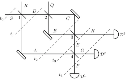
In the nested Mach-Zehnder interferometer (MZI) shown in Fig. 1, a particle from a source channel S

enters the outer MZI at beam splitter 1 and can pass through the lower armA, via a mirror, to beam splitter 4. However, the upper arm of the outer MZI is interrupted by an inner MZI, whose armsB andC, between beam splitters 2 and 3, connect the input channelsDandQto the output channelsEandH, withE going on to beam splitter 4. The reflectivities and phases of beam splitters 2 and 3 associated with the inner MZI

(3)

t0

t1

t2 _t₃

t4

R Q

S

D

E A

B C

H

G

F

D1

D2

D3

1 2

3

4

Figure 1: Nested Mach-Zehnder interferometer (MZI). The tilted solid lines are beam splitters numbered 1, 2, 3, 4; the double tilted lines are mirrors; the semicircles are detectors. The horizontal and vertical lines indicate different channels which are possible particle (photon) paths. The reflectivities and phases of beam splitters 2 and 3 associated with the inner MZI are chosen so that a particle entering through D will exit throughH and be detected byD3_{, rather than passing into}_E_{. The intersections of the dashed lines with}

the particle paths indicate possible locations of the particle at the successive timest0< t1< t2< t3< t4.

are chosen so that a particle entering throughD will exit throughH and be detected by D3_{, rather than}

passing into E. The output ports F and G of beam splitter 4 lead to detectors D1 _and

D2_{, respectively.}

(The detectors are denoted by a different font and labeled with superscripts to avoid any confusion with the

D channel and with the ket|D1iin (1).) The dashed lines in the figure indicate possible locations of the

particle at successive timest0< t1< t2< t3< t4 on its journey fromS att0 to one of the detectors.

LetTkj be the unitary time transformation that maps a ket at timetj to its counterpart attk. Here is a

suitable collection of unitaries (the choice is not unique); Tj,j−1 represents the action of beam splitterj in

Fig. 1:

T10: |S0i →α|A1i+β|D1i, |R0i → −β|A1i+α|D1i, |Q0i → |Q1i;

T21: |A1i → |A2i, |D1i →r|B2i+r|C2i, |Q1i →r|B2i −r|C2i;

T32: |A2i → |A3i, |B2i → −r|E3i+r|H3i, |C2i →r|E3i+r|H3i;

T43: |A3i →α|F4i+β|G4i, |E3i →β|F4i −α|G4i, |H3i → |H4i. (1)

The coefficients are real numbers:

0< α, β <1, withα2

+β2

= 1; r:= 1/√2. (2) The unitaries for larger time steps can be obtained using Tlj = TlkTkj, and for inverse time steps using

T_jk = T_kj† . One should think of kets such as |A1i or |B2i as normalized wave packets located in the

corresponding channels near the points where the dashed time lines cross the straight lines indicating the channels, and mutually orthogonal since they are far apart. In all there are fifteen of these kets in (1). While in principle eachTj,j−1should tell what happens to every one of them, (1) supplies all the information about

unitary time development that is needed for the present discussion. We are only interested in the situation in which the particle starts off in|S0iatt0, and is in either|A1ior |D1iat timet1, etc.

2.2 Where was the particle?

Suppose a particle that enters the outer MZI from S is later detected by D1_{. Where was it at earlier}

timest1, t2, andt3, when it was still inside the interferometer? Readers are invited to work out their own

answers before considering those discussed below. Here is the succession of states|ψji=Tj0|ψ0iobtained

by unitary time evolution using the transition amplitudes in (1), starting with|ψ0i=|S0i: |ψ1i=α|A1i+β|D1i, |ψ2i=α|A2i+rβ |B2i+|C2i

,

(4)

where|ψjicorresponds to the timetj in Fig. 1.

Li et al. in [3] (and Salih et al. in [5, 7]) assert that if D1 _{is triggered, then the particle was in channel}

F at t4 and in channelA at the earlier times t1, t2, andt3. In Sec. 3 we will show that this is, in a sense

which will be made clear, a correct answer. However, contrary to the claim in [7], it isnot a consequence of “standard quantum mechanics,” if by that one means what is found in standard textbooks. A student taking the final examination in Quantum 101 knows only that the quantum wave function develops unitarily in time until a measurement is made, leading to a mysterious collapse. And since at none of the times after

t0 and before the final measurement (at time t5) is |ψji confined to a single channel, the question of the

particle’s location cannot be answered using the textbook approach.

In practice, using quantum mechanics often requires going beyond, and sometimes forgetting, what is taught in textbooks, especially if one wants to take the talk of experimentalists seriously. Standard quantum mechanics as applied to the situation under discussion is best thought of as a series of rules for calculating the probabilities of certain macroscopic measurement outcomes given an earlier preparation, with|ψ(t)iat intermediate times a useful calculational tool, but otherwise not interpreted. This is a “black box” approach in that we (think we) understand preparations and measurements, while what goes on in between, inside the black box, is best not discussed. Those who dare open the box to try and figure out what is happening inside it risk going insane.1 _{But if we are to assess the claims and counterclaims mentioned in Sec. 1 we}

must open the box.

One line of reasoning which sounds plausible and will lead to the conclusion given in [3] can be worded as follows. The particle after it passed through beam splitter 1 was either in armAor in armD. If it was in armD, then because of the action of beam splitters 2 and 3 we know that it would have emerged in H, not inE. Had it emerged inH, thenD3

would have detected it, but since it was detected byD1

it was not detected byD3

. Thus att1the particle was surelynot in channelD, and hence it must have been inA, and

as there is no way the particle could escape fromAbefore reaching beam splitter 4, it must have been inA

at the timest1,t2, and t3.

Such reasoning has, as we shall see, arrived at a correct conclusion, but by a precarious route that is not altogether convincing. To begin with, what justifies treatingα|Ai+β|Dias “the particle was either in

A or it was in D”? Interpreting superpositions in this way is hazardous, and fails badly when applied to the double slit paradox. Next come some “if ... then” counterfactuals,2 _{and counterfactual reasoning in a}

quantum context has many pitfalls; see, for example, the exchange in [11, 12].

So one can understand why Vaidman [6] dismisses arguments of this sort as “a naive classical approach.” His own analysis in [2] reaches a different conclusion through employing the two state vector formalism (TSVF) [13, 14], plus some consideration given to weak and to strong nondestructive measurements. Let us begin with the TSVF; weak measurements will be discussed in Sec. 5.2. Along with the usual ‘forwards’ wave advancing unitarily in time from an earlier preparation, the|ψjiin (3), the TSVF employs a wave moving

‘backwards’ from a later measurement or, to be more precise, a property revealed by a later measurement. In the case at hand the later measurement result is detection byD1

, the corresponding property is|Fi, and one defines

|φji=Tj4|F4i, or hφj|=hF4|T4j; (4)

i.e., take the state|Fiand run it backwards through the beam splitters in Fig. 1. Since TSVF discussions generally usehφj|, we present the backward wave in this form:

hφ1|=αhA1|+βhQ1|, hφ2|=αhA2|+rβ(−hB2|+hC2|),

hφ3|=αhA3|+βhE3|, hφ4|=hF4|. (5)

Here the subscripts are time labels that correspond to those in (3).

Given the two state vectors, the bra-ket pair hφj| |ψji, Vaidman invokes a phenomenological principle

which says that at an intermediate timetj the particle can be said to be present in some channel provided

the amplitude for that channel in bothhφj|and|ψjiis nonzero; in particular this will produce what Vaidman

is present inhφ3|, |E3iis absent from |ψ3i. Similarly, at t1 the particle was inA but not in D. However,

att2 the particle was present in bothB andC as well as A, in disagreement with the claim in [3] that the

particle was inAand not elsewhere. Vaidman admits that his result seems a bit odd, as it is hard to imagine

1

A paraphrase of Feynman, p. 129 of [10].

2

(5)

how a particle could suddenly appear in B and C in the inner MZI when it was not present in channel D

connecting S to the inner MZI and then, equally mysterious, suddenly disappear so as to be absent from both E and H. As we shall see in Sec. 6, the TSVF approach interpreted in this way will sometimes give reasonable results, but can also mislead.

3 Consistent Histories Analysis

3.1 Introduction

Standard quantum mechanics as found in textbooks is far from a complete theory, and its rules do not cover situations which precede measurements, such as the one considered here. The consistent histories (CH) formalism is a systematic and consistent extension of textbook quantum mechanics. It gives the same results as the textbooks in the domain where the textbook rules can be properly applied, but in addition allows a paradox-free discussion of microscopic properties and events, such as those taking place in the nested MZI, for which textbooks provide little guidance. The CH approach, also known as decoherent histories, was developed to some degree independently by various researchers; some representative references are [15, 16, 17]. Short introductions will be found in [18, 19], an application to Bohm’s version of Einstein-Podolsky-Rosen in [20], and a discussion of how it relates to various quantum conceptual difficulties in [21]. A reasonably complete, albeit lengthy, treatment in [22] provides the basis for the material that follows.

The basic principles of the CH approach are: quantum properties as defined by von Neumann, unitary time development using the Schr¨odinger equation, stochastic dynamics using the Born rule and its extensions, and quantum histories. Measurements arenot included in this list, for in the CH approach measurements (see Sec. 5 below) are simply particular examples of quantum processes, all of which can analyzed using basic principles that make no reference to measurements. How these principles permit a detailed and consistent analysis of the nested MZI “which path” problem will be evident from the following discussion.

3.2 Quantum properties and sample spaces

According to von Neumann, Sec. III.5 of [23], a property of a quantum system at a particular time is represented by a subspace of the quantum Hilbert space, or, equivalently, the projector P (orthogonal projection operator) onto this subspace.3 _{Here ‘property’ is used in a restricted sense to mean a physical}

attribute (a proposition) which can be true or false; thus ‘energy’ is not a property, but ‘the energy is ǫ0’

or ‘the energy is less that ǫ1’ are examples of properties. The negation of a property, e.g., ’‘the energy is

greater than or equalǫ1’ for the case just mentioned, is also a property. In classical physics a property in the

sense used here always corresponds to a point or a set of points in the classical phase space, and its negation to all the points not in this set. Given two properties P and Q, the combinations ‘P AND Q’ and ‘P OR

Q’ correspond to the intersection and union of the two sets of points. If the sets corresponding to P and

Qdo not overlap, so the intersection is empty, ‘P AND Q’ is the empty set, the property which is always false, and whose negation, ‘NOT P’ OR‘NOTQ’, corresponds to the whole phase space, the property that is always true.

In quantum mechanics the negation of a propertyP (following von Neumann) is theorthogonal comple-ment of its subspace, with projector ˜P =I−P, whereIis the identity operator. However, ‘P ANDQ’ and ‘P ORQ’ only have a simple definition in the case in which the projectors commute, P Q=QP, and then

P Qis the projector representing ‘P ANDQ’, andP+Q−P Qis the projector representing (nonexclusive) ‘P

ORQ’. The headaches of quantum interpretation are all closely linked with the question of what to do when

P andQdonot commute. There are various approaches. The first, quantum logic [24], assigns a meaning to ‘P AND Q’ using the intersection of the subspaces, whether or not the projectors commute. However, quantum logic, as the name suggests, necessitates a change in the rules of reasoning in a fundamental way, and physicists have not yet had much success in making sense of the quantum world using the new rules; perhaps our intellectual children or grandchildren will do better. (See Sec. 4.6 of [22] for a very simple ex-ample showing why new rules are necessary.) A second approach is to replace or augment the Hilbert space

withclassical hidden variables which do not suffer from noncommutation troubles. However, the predictions

of hidden variables theories often differ from those of Hilbert space quantum mechanics, and when these difference are tested by experiment, the hidden variables approach always loses, so it seems unlikely that

3

A finite-dimensional Hilbert space will be adequate for our discussion, so the additional requirement that the subspace be closed is not needed.

(6)

this approach will prove useful in solving quantum mysteries. A third approach, employed by CH, limits discussions to cases where projectors commute: the conjunction ‘P ANDQ’ is only defined ifP Q=QP, in which caseP Qis the projector that represents the conjunction; but ifP Q6=QP, ‘P ANDQ’ is undefined, “meaningless” in the sense that this interpretation of quantum mechanics cannot assign it a meaning. Simi-larly, ‘P ORQ’ only makes sense whenP Q=QP. The CH approach retains the ordinary rules of reasoning

provided their application is suitably restricted to a single domain or “framework,” examples of which are

given below. A fourth approach is to go ahead and reason or calculate while ignoring, or at least paying little attention to, the noncommutation problem. A substantial body of quantum foundations literature is devoted to discussing the resulting paradoxes.

To make the discussion less abstract, consider the case of a two-state system, a spin-half particle for whichSz, the z component of angular momentum, can take the values of +1/2 or −1/2 in units of ¯h. Let

the projectors for the corresponding eigenstates be z+ ₌ |z+

ihz+

| and z−_{. They commute, since their}

product (in either order) is the zero operator, the quantum property that is always false, and their sum is

I, the property that is always true, so they constitute a quantum sample space orframework, call it theZ

framework. Similarly, the projectorsx+ _and_x− _{on the eigenstates of}_S

xconstitute theX framework. The

X andZ frameworks areincompatible in that the projectors in one do not commute with the projectors in the other, and the CH single framework rule prohibits combining them: ‘Sz = +1/2 AND Sx = +1/2’ is

meaningless, as is ‘Sz = +1/2 OR Sx = +1/2’. This is consistent with the fact that Sz can be measured,

andSxcan be measured, but, as the textbooks tell us, they cannot be measuredsimultaneously. The simple

explanation for the textbook rule is that these combinations ofSz andSx properties do not correspond to

Hilbert subspaces, so no quantum property exists which could be revealed by a simultaneous measurement. Standard (Kolmogorov) probability theory makes use of asample spaceof mutually-exclusive possibilities, one and only one of which can occur, be true, in any given situation. A quantum sample space is aprojective

decomposition of the identity(PDI), a collection of mutually orthogonal projectors which sum to the identity.

In the simplest situation each of the projectors has rank one: it projects onto a one-dimensional subspace (‘ray’) in the Hilbert space, and the sample space corresponds to an orthogonal basis of the Hilbert space. The

X andZ frameworks defined above are PDIs and thus quantum sample spaces. Two sample spaces (PDIs)

P andQarecompatible if every projector in one commutes with every projector in the other; otherwise they

areincompatible (as in the case ofX andZ defined earlier). When compatible,P andQpossess acommon

refinement made up of all distinct nonzero products of projectors fromP with projectors fromQ, which is

a PDI and thus a sample space. The single framework rule requires that logical or probabilistic arguments be based on asingle sample space; in particular one cannot use one sample space for part of an argument and then shift to another, incompatible sample space for another part, because this leads to paradoxes, such as those discussed in Ch. 22 of [22].

A crucial difference between ordinary (classical) applications of probability theory and its use in quantum mechanics is that in the latter there are often a variety of possible sample spaces which can be used to model a physical process, and whereas in some cases there is an “obvious” choice, in other cases the choice is far from obvious. Sometimes alternative choices of sample space are useful for different reasons, but there is no way of combining them; they are incompatible. The CH approach meets this diversity by noting that it is there, acknowledging that it is sometimes valuable to have two or more perspectives on a physical problem, and then insists on a strict enforcement of the single framework rule that prevents this diversity from leading to paradoxes. Because of the possibility of employing different frameworks it is important to be clear about which framework is being used in a particular discussion. Often this is evident from the context, but sometimes it is not, and then making the choice explicit can be helpful in order to avoid contradictions and paradoxes. Further comments on choosing frameworks will be found in Sec. 4.2, but first let us look at some examples.

3.3 Histories and consistency

The sample space of a classical stochastic process, such as a random walk or successive flips of a coin, consists of histories: sequences of properties at successive times. E.g., flipping a coin three times in a row can give rise to eight different histories, HHH, HHT, HTH, etc.; H for heads and T for tails. In quantum mechanics a history consists of a sequence of quantum properties, thus a sequence of projectors, at successive times. We will be considering histories for the MZI in Fig. 1, and in particular looking at projectors which in some way identify the location of the particle in different channels at successive times. Capital letters

(7)

example, the history

S0⊙A2⊙F4=S0⊙I1⊙A2⊙I3⊙F4 (6)

says that the particle started in channel S at t0, was in the A channel att2, and in the F channel att4.

The forms on the left and right sides are equivalent, because the identity operatorIprovides no information about the particle at the times t1 and t3. (One can interpret I3 as either the identity on the full Hilbert

space spanned by 15 kets, or simplyA3+E3+H3, the possibilities for the particle at t3; for our purposes

these are equivalent.)

The⊙symbol in (6) is a variant of⊗and is used to indicate a tensor product: the history is represented as a tensor product of projectors on ahistory Hilbert space

˘

H=H ⊙ H ⊙ · · · H (7)

constructed using copies of the Hilbert spaceHthat describes the system at a single time. A sample space

or family of quantum histories is a collection of projectors on ˘Hwhich sum to the identity ˘I, thus a PDI.

For example, the history (6) is a member of a family of four histories:

S0⊙A2⊙F4, S0⊙A˜2⊙F4, S0⊙I2⊙F˜4, S˜0⊙I2⊙I4. (8)

A tilde over a letter indicates negation, thus ˜A2 =I2−A2 =B2+C2, and ˜S0=I0−S0. Employing the

usual rules for adding tensor products of operators, the reader can easily check that the projectors in (8) sum to ˘I=I0⊙I2⊙I4, which means the same thing asI0⊙I1⊙I2⊙I3⊙I4when all five times are in view.

(Once again, replacing eachIj with the identity on the full Hilbert space of all 15 kets that appear in (1)

would make no difference in our discussion.)

We shall only be interested in cases in which the particle is inS at t0, and therefore we shall omit the

fourth history in (8) from the discussion which follows, which is equivalent to assigning it zero probability. The three histories that remain can be assigned probabilities using theextended Born rule, which, because they all begin with a pure stateS0, is most easily discussed usingchain kets, Sec. 11.6 of [22]:

|S0, A2, F4i:=F4T4,2A2T2,0|S0i=α2|F4i,

|S0,A˜2, F4i= 0, |S0, I2,F˜4i=β|H4i+αβ|G4i. (9)

Here the chain ket|S0, A2, F4iis obtained by applying to|S0ithe sequence of unitary operators and

projec-tors, T2,0, A2,T4,2, andF4, the same order as the events in the history (but from right to left). The other

chain kets in (9) are obtained by the same procedure. Note that chain kets are elements of the single-time Hilbert spaceH, not the history Hilbert space ˘H.

A family of histories is said to beconsistent if any two chain kets associated with distinct histories in this family are orthogonal to each other. For a consistent family the probability assigned to each history by the extended Born rule—to be precise, the probability conditioned on the initial stateS0—is the square of

the norm of its chain ket, the inner product of the chain ket with itself. The orthogonality just mentioned is referred to as aconsistency condition. If it is not satisfied the history family is said to be inconsistent, and no probabilities can be assigned to the corresponding histories. This means that an inconsistent family cannot be used in a probabilistic description of a quantum system; it is “meaningless” (lacks a meaning) within the CH formulation. (But see the additional comments in Sec. 4.3.)

From (9) it follows that the family in (8), with the final ˜S0 history omitted, is consistent. The

corre-sponding probabilities conditioned onS0are

Pr(A2, F4|S0) =α4, Pr( ˜A2, F4|S0) = 0, Pr(I2,F˜4|S0) =β2+α2β2, (10)

and in view of (2) they sum to 1. It then follows that

Pr(F4|S0) = Pr(A2, F4|S0) + Pr( ˜A2, F4|S0) =α4,

Pr(A2, F4|S0)/Pr(F4|S0) = Pr(A2|F4, S0) = 1. (11)

The last equality means that if the particle was inS at t0 and arrived inF at time t4 it was in channelA

(8)

3.4 History families using refinements

The family of three histories

S0⊙ {F4, G4, H4}, (12)

using a compact notation, involves only two times (or identity operators at the intermediate times), and is obviously consistent since the chain kets end in three mutually orthogonal states, so the extended Born rule reduces to the usual Born rule. A possible strategy for constructing consistent families is to take each of the histories in (12) and refine it by replacingIat some intermediate times with sums of two or more projectors, and then testing whether the result is consistent. We shall consider refinements of the subfamilyS0⊙F4,

but the same techniques can be applied to the other subfamilies S0⊙G4 andS0⊙H4. Each subfamily can

be refined, and its consistency checked, without regard to refinements of the other subfamilies; in particular, events at an intermediate time in one subfamily can be independent of those in a different subfamily. If a refinement yields an inconsistent (sub)family, further refinement will not restore consistency; one should try some other possibility.

We have already seen that the family (8) is consistent, which means that the (sub)family consisting of the first two of its histories,

FA: S0⊙ {A2,A˜2} ⊙F4=S0⊙ {A2, B2+C2} ⊙F4, (13)

a refinement ofS0⊙F4, is also consistent. This family can be further refined by adding events at timest1

andt3 to a family

FA′ : S0⊙ {A1, D1, Q1} ⊙ {A2, B2+C2} ⊙ {A3, E3, H3} ⊙F4, (14)

of 3×2×3 = 18 histories. However, the chain kets for all of them vanish, with the sole exception of the history

S0⊙A1⊙A2⊙A3⊙F4. (15)

Consequently,

Pr(A1, A2, A3|S0, F4) = 1, (16)

which is to say that the particle which entered the nested MZI throughS and left it throughF was in the

Achannel the entire time it was inside the interferometer. Also it was not in D1 orQ1 at time t1, nor was

it inE3 orH3 at timet3. The situation att2 is less clear, and will be discussed further below.

A different refinement ofS0⊙F4 yields the family

FB: S0⊙ {B2,B˜2} ⊙F4=S0⊙ {B2, A2+C2} ⊙F4. (17)

It is inconsistent, since the chain kets

|S0, B2, F4i=−(β 2

/2)|F4i, |S0,B˜2, F4i= (α 2

+β2

/2)|F4i, (18)

are obviously not orthogonal, at least when αand β are both positive, as assumed in (2). Hence further refining it, by replacingA2+C2with the pair{A2, B2}, will lead to an inconsistent family of three histories FABC : S0⊙ {A2, B2, C2} ⊙F4. (19)

The inconsistentFABC can also be obtained from the consistentFA in (13) by replacing ˜A2=B2+C2

with the pair{B2, C2}. Why should this make a difference? Here we encounter a very important conceptual

difference between quantum and classical physics. If projectorsB andCcommute, the quantum counterpart ofORin the sense of “BorCor both” is the projectorB+C−BC, and if, as in the present instance,BC= 0, the projectorB+C. But a Hilbert subspace B+C contains linear combinations such as 0.8|Bi −0.6|Ci

which belong to neither theBnor theCsubspace. In the classical world if something is “BorC”, assuming

B and C are mutually exclusive, we know at once that it is eitherB or else it is C. In the quantum world this is trueprovided one is using a framework that containsB and Cas separate projectors, but not if one is using the coarser description in which onlyB+C appears, notB andC separately. The sample spaces

{A, B+C}and{A, B, C}are not the same, and it is important to pay attention to which of these is in use. Some additional discussion of this very important point will be found in Sec. 4.1.

Yet another refinement ofS0⊙F4 is

(9)

with chain kets

|S0, C2, F4i= (β2/2)|F4i, |S0,C˜2, F4i= (α2−β2/2)|F4i. (21)

ThusFC will be inconsistent apart from the special case

α=p1/3, β=p2/3, (22)

for which the second chain ket in (21) is zero, allowing one to assign probabilities

Pr(F4|S0) = Pr(C2, F4|S0) =β4/4 = 1/9, Pr(C2|S0, F4) = 1, (23)

But does not the result Pr(C2|S0, F4) = 1 in (23), given the choice of coefficients in (22), contradict

the earlier result Pr(A2|S0, F4) = 1 in (11)? Can a particle emerging in channelF at time t4 have been

with probability 1 in both channel A and in channel C at t2? Is this not a contradiction? No, for in

the CH approach results obtained in two separate frameworks cannot be combined unless the frameworks themselves can be combined; once again the single framework rule. All the projectors for histories in FA

commute with those in FC, so there is a common refinement, FABC in (19). But this common refinement

is an inconsistent family, even for the special choice of parameters (22) for which FC is consistent. Hence

FA and FC are incompatible, or incommensurate if one wants a separate term for the situation in which

the inability to combine families arises from a failure of the consistency conditions, and thus the inability to assign probabilities, rather than the fact that the history projectors do not commute. The situation just discussed is an instance of the three box paradox of Aharonov and Vaidman [25]; see Sec. 22.5 of [22] for a discussion of how the CH approach resolves (or “tames”) this paradox. The three box paradox has certain features in common with the Bell-Kochen-Specker paradox [26], some versions of which are considered in Ch. 22 of [22].

4 Additional remarks

The previous discussion has employed some features of stochastic quantum time development using histories which call for a different type of thinking than is common in classical physics, and the following comments may be helpful in indicating how the CH approach avoids paradoxes and comes to reliable and non-contradictory conclusions about microscopic quantum events.

4.1 B

+

C

vs

_{

B, C

_}

The distinction between the sum B +C of two projectors and the projectors B and C considered as exclusive properties when BC = 0 was noted following (19), and can be illustrated using the well-known double slit experiment. A particle in an initial state|Sitravels towards the slit system and passes through it at an intermediate time before reaching the interference zone. LetBandC be projectors on two nonoverlapping regions of space, one containing the upper slit and one the lower slit, such that as it passes through the slit system the particle wavepacket is in the combined region corresponding to the projector

J =B+C. LetF be a projector on a region of destructive interference. A family

S⊙ {J,J˜} ⊙ {F,F˜} (24)

with four histories will be consistent, whereas refining it by replacing{J,J˜} at the intermediate time with

{B, C,J˜} will result in an inconsistent family. The projector J =B +C is noncommittal: “the particle passed through the slit system, but I tell you no more,” and is compatible with later interference, whereasB, “the particle passed through the upper slit,” andC, “it passed through the lower slit,” are not. Feynman in Ch. 1 of [27], with his superb physical intuition, knew that when discussing interference one should not try and identify which slit the particle passed through. One can think of the CH rule that excludes inconsistent families as a mathematical formulation of this intuition, allowing it to be applied not only to the double slit (for which see Ch. 13 in [22]), but to many other situations as well, and used by those of us whose physical intuition falls somewhat short of Feynman’s. Indeed, if one thinks of theB andCarms of the inner MZI in Fig. 1 as analogous to two slits, it is easy to understand why specifying them as exclusive alternatives can give rise to conceptual difficulties, as well as peculiar effects when using weak measurements, as discussed below in Sec. 5.2.

Yet another example is to think ofB andC as projectors on the ground state and first excited state of a quantum harmonic oscillator. Then bothB andC correspond to states of well-defined energies, and “B or

C” could be taken to mean that the oscillator has one energy or the other. On the other hand the subspace on whichB+C projects includes states which oscillate in time and do not have a well-defined energy.

(10)

4.2 Multiple frameworks

In quantum mechanics, unlike classical physics, there are often several distinct ways to describe a physical system and its time evolution, each of which is an acceptable application of quantum principles, but because of incompatibility they cannot be combined to form a single description. Which framework to use will be determined by the type of question one wants to address, and the single framework rule of CH helps guide this choice so as to achieve reliable results rather than inconsistencies and paradoxes. The single framework rule does not prohibit constructing multiple frameworks; what it forbids is combining incompatible frameworks to form a single description. Because there are multiple possibilities, it is important to be clear about which framework is being used in a particular discussion, something that may or may not be obvious from the context. Note that the choice of which framework to use is made by the physicist who is applying quantum principles to a particular situation; it isnotdetermined by some law of nature. In this respect it is analogous to the choice of a convenient coordinate system in classical physics with, however, the disanalogy that in classical physics all the information represented in a particular coordinate system can be transformed to a different coordinate system in a one-to-one fashion. By contrast, the information present in, say, the X

framework of a spin-half particle is entirely different from that in the incompatibleZ framework.

As an example, with reference to Fig. 1 we have been assuming, in agreement with previous literature, that a particle detected inD1 _{was at time}_t

4 in channelF. This is not the only possibility: the framework

of unitary time development that students learn in Quantum 101 employs a projector [ψ4] =|ψ4ihψ4|, where |ψ4i= T40|S0i is defined in (23). This unitary framework is a perfectly acceptable quantum description;

there is nothing wrong with it. But it cannot be used to discuss which channel the particle was in at t4

because [ψ4] does not commute withF4,G4, orH4. The CH approach allows an alternative framework in

which at a time just before the measurements take place the particle is in one of the channels leading to the detectors in Fig. 1, and in addition (see Sec. 5.1) it justifies the inference from detection by D1 _{to the}

particle’s having been inF att4, something which cannot be done using the textbook approach. So it should

come as no surprise that the familyS0⊙F4can itself be refined in various different ways. For example, the

family

S0⊙ {[φ2], I2−[φ2]}, F4, (25)

where [φ2] = |φ2ihφ2| is the projector corresponding to the the backward wave hφ2| defined in (5), is a

possible refinement ofS0⊙F4; we leave it as an exercise to show that it is consistent. Of course it is useless

for addressing the question of whether the particle is or is not in the A channel att2; for that purpose one

needs to useFA. Also, as noted in Sec. 3.4, both FA and FC are consistent, but mutually incompatible,

families for the choice of parameters in (22); the first is useful for deciding whether the particle was or was not inA, but cannot be used to discuss whether it was inC; the second can address the question of whether or not it was inC, but can say nothing aboutA.

Given this liberty in choosing families, one can ask whether this might not give rise to contradictions: different families assigning different probabilities to some event at an intermediate time, sayA2. However, as

long as probabilities are conditioned on the same set of events, e.g.,S0 andF4, the (conditional) probability

for an event at an intermediate time will be independent of the consistent family to which it belongs; see the discussion in Ch. 16 of [22]. For example, givenS0 andF4, the probability is zero that the particle was

inEat timet3. This can be shown using the familyS0⊙ {E3,E˜3} ⊙F4 (or by calculating the weak value of

E3at timet3using the method indicated in Sec. 6), and the answer is the same ifFAis refined by replacing

I3 with {E3,E˜3}. But if E was empty at time t3, how is it possible (see Fig. 1) for a particle arriving in

F att4 to get there fromC at t2, as must have been the case according to familyFC? The answer is that

refiningFC by replacingI3 with{E3,E˜3}makes it inconsistent, and thus when using FC it is meaningless

to ask whether the particle was in channelE at time t3. Once again it is the single framework rule, whose

central role in CH cannot be overemphasized, that prevents combining incompatible families to arrive at a contradiction. The quantum world is indeed weird from the point of view of classical physics, which is all the more reason why it must be analyzed using conceptual and mathematical tools that do not lead to contradictions and unresolved paradoxes.

As an example of multiple incompatible frameworks in a different context, consider an experiment in which a nucleus decays by emitting an alpha particle in an S wave (spherical symmetry), which is then detected some distance away. The experimenter will think of the particle as traveling along an almost straight path from the source to the detector, and the projectors appropriate to this description, corresponding to wave packets with a relatively narrow angular spread, do not commute with those that represent a spherical wave, so the two descriptions cannot be combined. In the CH approach both the spherical wave and the narrow

(11)

wave packet constitute perfectly acceptable quantum descriptions, and one or the other may be more useful for certain purposes.

The notion of multiple possible descriptions of the same experiment, of a sort that cannot be combined with each other, is very different from what one encounters in classical physics, so it may be helpful to try and identify the point at which classical intuition fails. In the world of everyday experience, where a classical approximation to quantum theory is adequate for all practical purposes, we tend to believe that at any instant of time there is a unique state of the world that is true or actual or real, even though no one knows what it is. This belief, elsewhere referred to asunicity (Sec. 27.3 of [22]), has a mathematical counterpart in the phase space of classical mechanics, where the state of a mechanical system at a given time is represented by one and only one point in the classical phase space. All properties (collections of points) that contain this point are true, while those that do not contain it are false. A Hilbert space is somewhat analogous to a classical phase space, and its one-dimensional subspaces, or rays, are analogs of the individual points in the phase space. But unlike two distinct points in the phase space, two different rays do not represent mutually exclusive physical properties unless they are orthogonal to each other. To put the matter differently, if one thinks of a single ray as representing the “real” state of the quantum world, and that all subspaces that contain it are true, while those orthogonal to it are false, this leaves many subspaces that belong to neither category, and thus are neither true nor false. Hence if the real world is best described using a quantum Hilbert space and its subspaces, rather than a classical phase space, unicity does not correspond to physical reality.

4.3 Dynamics and consistency

It is worth noting that consistency depends not just on the history projectors, but also on the unitary dynamics, the Tkj, used to compute the chain kets. A family which is inconsistent for a particular unitary

dynamics may be consistent for a different dynamics. Thus FC in (20) is in general inconsistent, but for

the special choice ofα andβ in (22) it is consistent. A more drastic change in the dynamics would be to eliminate beam splitters 3 and 4 in Fig. 1, in which case the family

S0⊙ {A2, B2, C2} ⊙ {F4, G4, H4} (26)

will be consistent, in contrast to the inconsistent familyFABC in (19). Since the particle only encounters

beam splitters 3 and 4 after t2, one might be tempted to suppose that the future is somehow influencing

the past. But the change is in what can inferred about past properties, the particle’s location att2, from

later measurement outcomes, and it is not unreasonable to suppose that altering the unitary time evolution connecting the two will make a difference.

There are many other examples. An inconsistent family for an isolated system may become consistent if that system interacts with an environment. Decoherence can have this effect, and so can subjecting a system to external measurements. In the CH approach measurements must themselves be described, at least in principle, using quantum mechanics, so what can be consistently said about a system in the presence of a measurement may or may not be possible when there is no measurement. See the discussion in the paragraph following (35) in Sec. 5.2 for a particular example.

5 Measurements

5.1 Introduction

A quantum measurement is a process by which information about some microscopic property or behavior of the system of interest is amplified so that it can be represented through distinctive macroscopic properties of a measuring device, “pointer positions” in the archaic but picturesque language of quantum foundations. In textbook quantum mechanics students learn how to calculate a probability for a microscopic property, such as Sz = +1/2 for a spin half particle, by using the Born rule applied to a ket or density operator

for the microscopic system, and are told that this is the probability of this property if it is measured. The CH approach, see Chs. 17 and 18 of [22], supplies the steps missing from textbooks by providing a complete, albeit schematic, quantum mechanical description of the entire measurement process, assuming an appropriate interaction between the apparatus and the system to be measured. The infamous measurement problem of quantum foundations, the fact that unitary time development will typically leave the apparatus in a superposition of pointer states, is disposed of by using a framework of macroscopic properties, an

(12)

appropriate PDI corresponding to different pointer positions. The second measurement problem, inferring the prior microscopic state from the final pointer position, is taken care of by using a framework that includes an appropriate microscopic PDI at a time just before the measurement takes place, and then using standard probabilistic reasoning to infer (retrodict) the earlier microscopic state from the later pointer position. In the case of the nested MZI in Fig. 1 one can think ofD1

,D2

andD3

as constituting a single measurement device whose “pointer” is whichever device has detected the particle, while the microscopic PDI consists of {F4, G4, H4}, the possible locations of the particle just before detection. This is how the CH approach

justifies the inference from detection byD1_{to the particle having been in}_F _at_t 4.

5.2 Weak measurements

Aweak measurement in contrast to astrongorprojective measurement of the type discussed above, is one

in which the system to be measured (in our case the particle or photon) interacts weakly with the measuring apparatus, so that on average neither the apparatus nor the particle is strongly perturbed. Hence extracting useful information requires repeating the experiment a large number of times. (We are not considering the case in which a large number of weak measurements are carried out in succession on a single system.) Even though the interaction is weak it can still on rare occasions produce a strong effect on the measured system; see, for example, Feynman’s discussion in Sec. 1-6 of [27]. Though outcomes of weak measurements are often analyzed in terms ofweak values, as in [3], this is not necessary. The mathematical definition (see (36) below for an example) of a weak value is clear, but its physical significance is obscure, and therefore we shall make no use of it, but instead employ a more straightforward interpretation of the weak measurement outcome.

To study the passage of the particle through the nested MZI, assume that attached to each channel is a two-state system, a qubit probe, which is initially in its “ground” state |0i. The probes in channelsA,

D, B, C, E are labeled by the corresponding lower case letters a, d, b, c, e. In addition there is a special probewto detect a particle passing throughB+C without distinguishing B from C; recall the discussion in Sec. 4.1. No probes are needed for channelsF, G, and H, as these terminate in strong measurements. The passage of a particle through channelP with probepresults in a unitary time development

|Pi ⊗ |0ip→ |Pi ⊗ ζ|0ip+η|1ip

; η=√ǫ , ζ=√1−ǫ, (27) whereǫis a very small number, think of 1/10000, whereas if the particle does not pass through theP channel the probe remains in the state|0ip. For interaction with theB+Cprobew, use (27) twice, once withP =B

and once with P =C, with p=win both cases. It will be convenient to label states of the entire system of probes using a symbolκ, whereκ=ois the initial state with no probes excited,κ=dbmeans probesd

andb are excited and the rest are not, and so forth. Thus when the particle passes through channelP the result is

|Pi ⊗ |κi → |Pi ⊗ ζ|κi+η|κpi

, (28)

whereκpmeanspifκ=o,bpifκ=b, and so forth.

After a given run is finished each probe can itself can be subjected to a strong measurement in the|0i,|1i

basis to determine its value. A probe state|1iindicates that the particle was in that channel (or inB+C

for probe w), but if the state is |0i one learns nothing: the particle might have been in the channel, but if so it left no trace. Note that the process of measuring the probes, which takes place after the particle has completed its path through the trajectory, has no effect upon that trajectory, since the future does not influence the past; instead, the measurement yields information about the state of affairs at the earlier time. One can then ask: given that the particle emerged inF orGorH (as indicated by its triggeringD1

orD2

orD3

), which, if any, of the probes registered its passage through one of the preceding channels? Sinceǫ is very small, the answer will usually be “none at all,” but occasionally one of the probes will be excited, and much less frequently two, or even three probes will have been excited in the very same run, hence providing information on the trajectory of a single particle during that run.

The discussion is simplest for the case in which the B andCprobes are absent, but theB+C probe is present, along with the probes for A, D, and E. Let|Ψji, the counterpart of |ψjiin (3), be the result of

unitary time evolution of the particle together with the system of probes up to timetj, starting from the

state|Ψ0i=|S0i ⊗ |oi, and assuming that at time tj the interaction with the corresponding probe has just

taken place. All the information of interest to us will be present at timet4, and it is convenient to write |Ψ4iin the form

|Ψ4i=

X

κ

(13)

A straightforward calculation yields

|Φo_i₌_ζα_|_A_¯

4i+ζ2β|H4i, |Φai=ηα|A¯4i,

|Φdi=|Φwi=ζηβ|H4i, |Φdwi=η2β|H4i, (30)

and all the other|Φκ_i_{, such as}_|_Φad_i_{are zero. We have used the abbreviation}

|A¯4i=α|F4i+β|G4i=T43|A3i (31)

for the state att4which results when|A3ipasses through the final beam splitter. One can use these results

to derive probabilities conditioned on the initial state|Ψ0i, such as

Pr(F4, a) =|hF|Φai|2=ǫα4,

Pr(F4, o) =|hF|Φoi| 2

= (1−ǫ)α4

,

Pr(F4) =α4, Pr(a|F4) =ǫ. (32)

That is, given that the particle emerged inF att4(was detected by D1), there is a conditional probability

of 1−ǫthat no probes were triggered,ǫthat theaprobe was triggered, and zero that any other probe was triggered. In particular, thed,w, andeprobes were never triggered if the particle emerged inF, indicating that this particle was never in theDor theEchannel, and never in theB+Cchannel system. The conclusion is the same if the particle emerged inG. All of this is consistent with the discussion of particle trajectories in Sec. 3.3. And it agrees with the conclusion reached by Li et al. [28], who suggested a possible, albeit rather difficult, way to realize thewprobe in an actual experiment. If, on the other hand, the particle emerged in

H, there is a probability of orderǫthat either thedor thewprobe was triggered, and a probability of order

ǫ2_{that both probes were triggered in the same run. The}_e_{probe is never triggered. Again, this is just what}

one might expect.

Next consider the situation in which the B andC probes are present, but theB+Cprobewis absent. A straightforward but somewhat tedious calculation shows that the nonzero|Φκ_i_{in (29) are:}

|Φoi=ζα|A¯4i+ζ2β|H4i, |Φai=ηα|A¯4i, |Φdi=ζηβ|H4i, |Φb_i₌1

2ζηβ(−ζ|E¯4i+|H4i), |Φ

db_i_{= (}_η/ζ₎_|_Φb_i_,

|Φc_i₌1

2ζηβ(ζ|E¯4i+|H4i), |Φ

dc_i_{= (}_η/ζ₎_|_Φc_i_,

|Φbe_i₌_−|_Φce_i₌₋1 2ζη

2

β|E¯4i, |Φdbei=−|Φdcei=−(η/ζ)|Φbei, (33)

where|A¯4iis defined in (31), and

|E¯4i:=β|F4i −α|G4i=T43|E3i, (34)

is the state produced when|E3ipass through beam splitter 4.

Using these results one can determine which probes have been triggered and with what probability if the particle emerges in one of the channelsF,G, orH. For our purposes the essence of the matter can be summarized in two lists: the first indicates which probes can have been excited if the particle emerges inH

(detected byD3

); and the second gives this information if the particle emerges in either F or G(detected byD1_or

D2_):

H: o, d, b, c, db, dc,

F ORG: o, a, b, c, db, dc, be, ce, dbe, dce. (35) Assuming neitherαnorβ is very small, the probability that a setκof probes was excited is of orderǫ|κ|_{: 1}

if no probes have been excited; andǫ,ǫ2_{, or} _ǫ3 _{in the case of one, two, or three probes excited during the}

same run.

The H list in (35), which does not contain a or e, is consistent with the idea that when detected by

D3

the particle was earlier in the upper arm of the nested MZI and never in either A or E. This is not surprising. In runs in which the particle was detected byD1

or D2

, so emerged from the MZI in F or G, a single probe aor b or c was excited with a probability of orderǫ, but neverd or e, a result which could be taken to support Vaidman’s assertion, Sec. 2.2, that this particle was inB orC as well as inA, but was never inD orE. However, the coincidences, two or more probes triggered during a single run, agree with

(14)

the alternative explanation given in [3]: the perturbing effects of a weak measurement inB or inC. Thus if thebprobe was excited, it indicates that the particle was in the B channel, not theCchannel (note thatb

andcnever appear in coincidence). This spoils the coherence between theB andC channels, and allows the particle to emerge from the inner MZI with equal probability inEor inH. If it emerges inEthere is a small probability (another factor ofǫ) that it will trigger theeprobe before reaching eitherF orG. This explains thebecoincidences, and the fact that eis never excited unless preceded byb or c. The same reasoning can explain the db, dbe, ce, dc, and dce coincidences. In the limit ǫ→ 0 this symmetry-breaking effect of the

b and cprobes will go to zero, and the situation will resemble the one discussed previously in which these probes were absent and only thewprobe was present. Hence the weak measuring results are consistent with the conclusions in Sec. 3.3 based on the CH analysis, where there were no weak measurements, once one has taken into account the fact that measurements, even when they are weak, can sometimes perturb a quantum system.

The situation in which theB,C andB+Cprobes are present along with those forA,D, andEleads to longer and messier expressions, since there are many moreκfor which Φκ _{is nonzero. However, the results}

are consistent with what one would expect from the preceding analysis. In cases in whichb orcare excited,

w can also appear (with a probability smaller by orderǫ), but ifw is not accompanied by bor byc in the same run, it also is not accompanied by e, i.e., the particle always emerges from the inner MZI in channel

H.

The reader might wonder whether replacing the qubit probes employed here with Gaussian probes of the sort often employed in the weak measurement literature would lead to different conclusions. The answer is that it would not. The easiest way to see this is to note that the interaction specified by (27) and (28) gives rise, so far as the particle (photon) is concerned, to a noisy quantum “phase damping” or“phase flip” channel (see, e.g., Sec. 8.3.6 of [29]), whereas the probe forms thecomplementary channel, as defined, for example, in [30]. Since the phase damping channel has only two Kraus operators, the simplest complementary channel is two dimensional, thus a qubit channel. A standard result in quantum information theory is that the direct (phase flip) channel determines a unique complementary (probe) channel up to a unitary transformation on the latter [30]. Thus a Gaussian probe cannot carry away more information than a qubit probe, though analyzing the Gaussian probe might be less straightforward.

6 Two State Vector Formalism

The connection between the two state vector formalism (TSVF) [13, 14] and the CH approach can be conveniently discussed using the formula

hQiw=hφ2|Q|ψ2i/hφ2|ψ2i (36)

which defines the weak value [31] of the operator Q in terms of bra-ket pair hφ2| |ψ2i at the time t2. In

particular

hF4|S0, P, F4i=hφ2|ψ2ihPiw (37)

relates the chain ket, see (9), for the historyS0⊙P ⊙F4 to the weak value of the projectorP. Using|ψ2i

from (3) andhφ2|from (5) one obtains:

hA2iw= 1, hB2iw=−β2/2α2, hC2iw=β2/2α2. (38)

Sincehiw is linear andhIiw= 1, it is the case that

hPiw+hP˜iw= 1, (39)

with ˜P =I−P. Consequently, the family S0⊙ {P,P˜} ⊙F4 will be consistent—one of the chain kets, see

(37), is zero—ifhPiw is 1 or 0, but will be inconsistent in all other cases. Thus an immediate consequence

of (38) is that the familyFA withP =A2, see (13), is consistent for all values ofαandβ;FBwithP =B2,

see (17), is never consistent for α and β satisfying (2); andFC with P = C2, see (20), is only consistent

whenβ2

/2α2

= 1, i.e., for the special values in (22).

Vaidman’s principle, as noted in Sec. 2.2, is that the particle is present (in some sense) whenever the weak value of the projector representing the channel is nonzero, and absent when the weak value is 0. The CH approach says the particle is present when the weak value of the channel projector is 1, is absent when the weak value is 0, and otherwise its presence or absence cannot be discussed, since the history family is

(15)

inconsistent, so one cannot assign probabilities. The same comparison can be made if the intermediate time ist1 ort3, using the bra-ket pair for this time, and assuming a family of histories defined att0,t4, and with

only one nontrivial (the event is not simplyI) intermediate time. Consistency conditions (orthogonality of chain kets) can also be discussed for histories with additional nontrivial intermediate times, but for these there is no obvious connection with the TSVF.

7 Counterfactual Communication

While the preceding analysis disagrees with Vaidman’s claims about the path of a particle in a nested MZI, it also casts serious doubt upon the counterfactual communication claim of Salih et al. [5], and, indeed, for much the same reason: the impossibility of includingB andCseparately, rather thanB+C, at timet2

in a consistent family of histories. The nature of the difficulty is most easily seen in the reply of Salih et al. [7] to Vaidman’s criticism [6] of their earlier work in [5]. This reply contains a figure similar to our Fig. 1, albeit rotated by 45◦_{, and uses identical labels for channels} _A_,_B_,_C_,_D_{, and}_E_{, and similar labeling for the}

detectors, apart from subscripts in place of our superscripts. With reference to this figure Salih et al. [7] say that:

A click at D1 implies that the photon should have followed pathA, and the probability of its

existence in the public channel is zero.

The “public channel” in the counterfactual communication protocol is the one by which Bob communi-cates with Alice. In terms of Fig. 1, all the beam splitters lie in Alice’s domain, and only theC channel mirror belongs to Bob. Thus for our purposes the public channel is the same as the C channel. Let us assume in addition that detection by D1, i.e., D1, is equivalent to the particle emerging from the MZI in

channelF, and consider three propositions expressed in the notation of Fig. 1: P1. The particle was inS att0and inF att4.

P2. The particle was inAat t2

P3. The particle was not inCat t2.

The quotation from [7] given above can be summarized as: P1 implies P2, P2 implies P3, and therefore P1 implies P3.

Let us now examine this argument. The step from P1 to P2 can be justified using the family FA, (8),

since the final equality in (11) is Pr(A2|S0, F4) = 1. The trouble is with the step from P2 to P3. To

understand why, it is helpful to insert between P2 and P3 the proposition P2´. The particle was not inB+C at t2.

Since B2+C2 = ˜A2 is in FA and Pr(B2+C2|S0, F4) = 0, P2´ is a direct consequence of P1 as well as

implied by P2. However, to get from P2´ to P3 it is necessary to go from “notB+C” to “not C”, and this requires refining the framework containing the projectorB+Cto one containing bothB and C. This nontrivial requirement was noted at the end of Sec. 3.3, and discussed further in Sec. 4.1. In the present context such a refinement would lead to the inconsistent family FABC in (19), so it is not allowed.

Note that if one were only concerned about events at timet2the step from P2 or P2´ to P3 would cause

no difficulty; one would simply refine{A2, B2+C2} to {A2, B2, C2} and employ the latter to reason from

the presence of the particle in Aat time t2 to its absence fromC. The difficulty arises because one wants

to infer P3 from P1, and P1 contains information about events att0 andt4. The single framework rule says

that cannot simply forget the framework used to infer P2 (or P2´) from P1 when carrying out the next step from P2 (or P2´) to P3. It is at this point where classical reasoning is inadequate. The single framework rule is not part of the logic of classical physics because it is never needed: all of classical physics, as seen from a quantum perspective, requires only a single framework. But in the quantum world one has to modify classical reasoning if one is to reach reliable conclusions.

Could one get from P1 to P3 by a direct route that does not include P2? The coarsest framework that includes C2 along with S0 and F4, and hence both the premises in P1 and the consequences in P3, is FC,

(20), and in general this family is inconsistent, so it cannot be used to assign a meaningful probability to

C at t2. Only for the special choice of parameters in (22) is FC consistent, and in that case one can use

(16)

in (22) P1 implies not that P3 is true, but that it is false! (As noted at the end of Sec. 3.3, this result obtained using FC does not contradict Pr(A2|S0, F4) = 1 obtained using the familyFA, which is valid in

general, including the choice of parameters in (22), because FA and FC are incompatible—to be precise,

incommensurate—families, and the single framework rule means they cannot be combined.)

Thus the inference from P1 to P3 does not satisfy the rules for quantum reasoning, and one cannot conclude that a particle emerging in channel F was earlier absent from channel C. Hence the argument employed by Salih et al. in [7] is not valid. To be sure, the figure in [7] was presented as a simplified example to illustrate the point the authors were trying to make; their full protocol is much more complicated. But if the reasoning applied to this simplified example is defective in the manner just discussed, it is hard to accept their claim about the more complicated protocol unless and until it has been justified by better arguments than have been presented up to now.

One may add that the very notion of counterfactual communication seems problematical in light of the fact that it is impossible to transmit information between quantum systems which do not interact with each other [32]. Of course, “interaction” is not the same thing as sending particles, though it is hard to see how in the protocol under consideration there could be an interaction sufficient to convey information in the complete absence of particles (photons) passing from Bob to Alice. In addition, the claim in [5] is not that precisely zero particles are involved, but rather that the number in the Bob to Alice channel can be arbitrarily small in an asymptotic limit of a large number of opportunities for the photon to pass back and forth. But then a proper analysis of the situation requires appropriate quantitative estimates based on sound quantum principles.

8 Conclusion

The possible paths followed by a particle (photon) that enters the nested Mach-Zehnder interferometer in Fig. 1 through channelS and later emerges in channelF to be detected byD1_{have been analyzed using}

consistent histories. The consistent familyFAin (13) and its refinement in (14) leads to the conclusion (16)

that the particle was in theAarm of the interferometer at all times while inside the interferometer, and was not in the small interferometer in the sense that zero probability is assigned to the projectorB+Cat time

t2. This result agrees with Li et al. [3] rather than Vaidman [2].

However, closer inspection shows that this result is not altogether straightforward; one needs to pay attention to certain subtleties. Assigning zero probability toB+Cat timet2conditional onS0andF4does

not by itself mean that zero probability can be assigned toB andC separately. WhereasB+C at timet2

is part of a consistent family FA, (13) (and FA′, (14)), refining FA by replacing the projectorB+C with

the pair {B, C}, i.e., treatingB and C as mutually exclusive alternatives, leads to an inconsistent family. This is a case in which straightforward classical reasoning in a quantum context leads to incorrect results. The difference between the projectorB+C and the pair {B, C} is discussed Sec. 4.2; while Sec. 7 shows in detail how the reasoning process fromS0 andF4 to “notC2” breaks down, and why this has important

implications for the claim of counterfactual communication.

For the special choice of beam splitter parameters in (22), ignoring the single framework rule leads to a paradox, Sec. 3.4: given the same conditions, S at t0 andF at t4, the consistent family FA leads to the

conclusion that the particle was in A at t2, whereas the equally consistent family FC locates the particle

at t2 in C. This is an instance of the three box paradox in quantum foundations; details of how the CH

approach resolves it (perhaps better, “tames it”) will be found in Sec. 22.5 of [22]. Here it suffices to note thatFA andFC are incompatible (to be more precise, incommensurate) families that cannot be combined,

so the contradiction that arises when using classical reasoning is eliminated when proper quantum principles are applied.

Both Vaidman [2] and Li et al. [3] have appealed to the weak values produced by weak measurements to determine the particle’s path. The analysis in Sec. 5, which uses qubit rather than Gaussian probes, and employs a straightforward interpretation of the results rather than weak values (whose connection with actual particle properties is quite obscure), supports the conclusions reached in Sec. 3 using the familyFA:

at the timet2 the particle was inA. It is worth noting that even a very weak interaction between the probe

and the measured system can on rare occasions produce very large perturbations of the latter. And also that for the fairly simple situation considered here, qubit probes provide just as much information as Gaussian probes, and in a form which is easier to interpret.

The comparison of the two state vector formalism and the consistent history approach in Sec. 6 throws additional light on the disagreement, mentioned in the introduction, between Vaidman and Salih et al. on the

Particle Path Through a Nested Mach-Zehnder Interferometer

arXiv:1604.04596v2 [quant-ph] 17 Aug 2016