THE ROLE OF INTERANNUAL RAINFALL VARIABILITY ON
RUNOFF GENERATION IN A SMALL DRY SUB-HUMID
WATERSHED WITH DISPERSE TREE COVER
S. SCHNABEL*, Á. GÓMEZ-GUTIÉRREZ
Grupo de Investigación GeoAmbiental, Universidad de Extremadura, Cáceres, Spain.
ABSTRACT. Recent studies in small experimental catchments under
Mediterranean-type climate revealed a complex hydrological catchment response, presenting saturation excess runoff generation and, to a minor degree, infiltration excess flow. Many of these catchments, however, belong to areas with sub-humid or humid Mediterranean climate. Catchment studies were carried out since 1991 in savannah-like grazed land (dehesas), which are widespread in south-western Spain, and also elsewhere in the Mediterranean. Albeit knowledge gained by previous studies, no thorough analysis has been carried out on the temporal variation of discharge production using the complete dataset. The objectives include i) an analysis of the temporal variation of discharge and rainfall at different temporal scales, ii) exploration of the role of antecedent soil moisture conditions in runoff production, iii) empirical modeling of rainfall-runoff relationships at the event scale and iv) definition of the importance of interannual rainfall variation on discharge production. The analysis were based on rainfall and runoff which were monitored at a time resolution of 5 minutes and periodically measured soil moisture from various depth in the valley bottom. Regression analysis as well as the comparison of hydrographs illustrate on the importance of antecedent rainfall conditions. Soil moisture in the valley bottom was crucial to understand the hydrological behaviour of the catchment. A soil moisture threshold of 0.37 m3m-3 was defined above which runoff coefficients
increase sharply. This situation is reached with 170 mm of antecedent rain falling in a continuous way. The results indicate that saturation excess flow and preferential subsurface flow processes are responsible of most of the runoff generated. Hortonian type overland flow dominates under dry soil conditions and is produced by high intensity rainfall.
Mediterranean, discharge was very low. Runoff is highly concentrated in time with 10% of the months accounting for 85% of total discharge.
El papel de la variación interanual de la precipitación en la generación de escorrentía en una pequeña cuenca de clima sub-húmedo seco con arbolado disperso
RESUMEN.Los estudios más recientes en pequeñas cuencas experimentales de ambiente mediterráneo muestran una respuesta hidrológica compleja, con esco-rrentía de saturación por exceso y, en menor medida, escoesco-rrentía debida a flujo por exceso de infiltración. Sin embargo, la mayor parte de estas cuencas presen-tan climas de tipo mediterráneo húmedo o sub-húmedo. En los ambientes adehe-sados que predominan en el Suroeste peninsular y otras zonas del Mediterráneo, se desarrollan estudios a escala de cuenca desde 1991. A pesar del conocimiento adquirido en estos trabajos, aún no se ha llevado a cabo un análisis profundo de la variación temporal en la producción de caudal utilizando las bases de datos dis-ponibles. Los objetivos de este trabajo incluyen i) analizar la variación temporal de la descarga, el caudal y la precipitación a diferentes escalas temporales, ii) analizar el papel de las condiciones de humedad antecedente del suelo en la pro-ducción de escorrentía, iii) modelizar de forma empírica las relaciones precipita-ción-escorrentía a escala de evento y iv) determinar la importancia de la variabilidad interanual de la precipitación en la producción de caudal. Para el desarrollo del trabajo se utilizaron la precipitación y la descarga acuosa, regis-tradas con una resolución de 5 minutos, así como la humedad del suelo medida periódicamente en los suelos de las vaguadas y a diferentes profundidades. El análisis de regresión, así como la comparación de los hidrogramas, muestran la importancia de las condiciones antecedentes de humedad. La humedad del suelo en los fondos de valle resultó crucial para comprender el comportamiento hidro-lógico de la cuenca. Se definió un umbral de 0.37 m3m-3de contenido de humedad
medi-terráneos, la descarga se reduce enormemente. La mayor parte de la descarga generada, el 85%, se concentra en el 10% del tiempo.
Key words: discharge, rainfall, soil moisture, empirical modelling, drought, dehesa. Palabras clave: escorrentía, precipitación, humedad del suelo, sequía, modelo empíri-co, dehesa.
Enviado el 17 de diciembre de 2012 Aceptado el 26 de enero de 2013
* Correspondencia: Grupo de Investigación GeoAmbiental, Universidad de Extremadura, Cáceres, Spain. E-mail: [email protected]
1. Introduction
In regions with a marked seasonality in climate, such as the Mediterranean, the rainfall–runoff relationship is reported to be more complex and variable than in humid regions (Beven, 2002). Under Mediterranean-type climate, runoff generation has been described to switch from a Hortonian type during the dry periods to one dominated by subsurface stormflow and saturation excess flow during short humid periods, more typical of humid climates.
In several drainage basins with Mediterranean mountain climate rainfall-discharge relationships at the event scale were observed to be poor, attributed to the complexity in the generation of runoff (Gallart et al., 2002; García-Ruiz et al., 2005). Llorens (1991) and Llorens and Gallart (1992) already showed that the response of these catchments is largely driven by antecedent conditions than by rainfall intensities and further research showed that during the year, the dominant runoff generation mechanisms change gradually, as a result of both varying catchment antecedent wetness conditions and changing rainfall events characteristics (Gallart et al., 2002).
Variability of the catchment hydrological response and the seasonal dynamics of runoff-contributing areas were investigated in the Catalan Pyrenees by Latron et al. (2008) and Latron and Gallart (2007) and by Lana-Renault et al. (2007) in the Central Pyrenees. These studies showed that under humid catchment conditions discharge generation was enhanced by subsurface flow and excess flow produced in saturated areas.
The role of antecedent moisture conditions was also demonstrated for a semiarid catchment in Murcia by Castillo et al. (2003). The authors report that the hydrological response of high intensity, low frequency storms is independent of the initial soil water content. On the other hand, the antecedent soil water content is an important factor controlling runoff during medium and low intensity storms, a type of rainstorm that is relatively frequent in semiarid areas.
very similar characteristics as the Parapuños catchment, subject of the present paper. During dry conditions only rainstorms with high amounts and high intensity generate discharge rapidly and with storm hydrographs characterized by short duration and small volumes of water. Under humid antecedent conditions the hydrographs also show a rapid rise, but being more prolonged, with higher total amount of discharge and higher runoff coefficients. This contrasting runoff generation was explained by varying hydrological catchment response, with Hortonian overland flow dominating during dry conditions and saturation excess flow during humid conditions. Of importance is the sediment fill in the valley bottoms contrasting with the shallow soils developed on the hillslopes, common in the peneplain landscapes of south-western Iberian Peninsula. Genesis and quantity of runoff (Hortonian or saturation) measured at the outlet depend on the antecedent moisture conditions of the valley bottoms because of their water-retention capacity (Ceballos and Schnabel, 1998).
On the other hand, rainfall simulation experiments carried out on microplots in Guadalperalón evidenced the existence of preferential flow in soils (Cerdà et al., 1998). Hydrological modelling of the Parapuños catchment by Maneta et al. (2008) showed that the total runoff has a fast component attributed to surface runoff, and a slow component. Simulating this combined process proved to be difficult. The simulated fast component, if modelled as surface flow, had to be slowed down with very high Manning’s n values, while the simulated groundwater release to the channel was too slow compared to measured fluctuations in piezometers. A recent study by van Schaik
et al. (2008) in the Parapuños catchment including a detailed analysis of soil moisture content and water level pointed out that, depending on catchment conditions and rainfall characteristics, between 13 to 80% of the catchment runoff may be produced by subsurface stormflow instead of by surface runoff. A large connected macropore network is anticipated to exist, which can transport water laterally regardless of the soil moisture content of the matrix. Under dry conditions the macropores loose a lot of water to the matrix, but can also transport water as rapid subsurface stormflow. Under near saturated conditions there is little infiltration to the matrix and most of the water will become subsurface stormflow.
The catchment has shallow soils overlying an almost impervious material and dries out completely over the summer, hence a full year’s water balance can be established without accounting for differences in soil water storage. Over the year, i.e. from September to September, the total precipitation must be equal to the sum of runoff and evapotranspiration (Ceballos and Schnabel, 1998).
1. Characterizing the temporal variation of discharge and rainfall during the study period at different temporal scales (event, month, year).
2. Exploring the role of antecedent soil moisture conditions in runoff production. 3. Empirical modelling of rainfall-runoff relationships at the event scale.
4. Comparing long-term rainfall data with data gained in the study catchments giving special attention to dry and humid periods.
5. Defining the importance of interannual rainfall variation on discharge production.
2. Study Area
Research has been carried out since September 2000 in the Parapuños experimental watershed located in the Spanish region of Extremadura (Fig. 1). The basin has an area of 99.5 ha and is representative of a savannah-like rangeland termed dehesa,which is widespread in the south-western part of the Iberian Peninsula. A review of soil and water dynamics of dehesas, including the role of trees and soil degradation, is found in Schnabel et al. (in press). Physiographically, the area, belonging to the Tagus river basin, forms part of an extensive erosion surface (Gómez Amelia, 1985) with an undulating topography. The dominant rocks of the Parapuños catchment are schist with residual pediments found in the highest parts of the basin. The altitudes of the catchment range from 361 to 453 m a.s.l. and an average of 396 m a.s.l. Mean slope is 7.9%, ranging from almost flat surfaces in the valley bottoms to 12% at the hillslopes. The main channel is a second order stream, which in the lower part of the catchment is incised into alluvial sediments of approximately 1 m thickness, reaching the underlying schist. The channel and its tributary can be classified as gullies due to the active erosion taking place.
The soils in the catchment developed on schist are shallow (< 30 cm), have low organic matter content and can be classified as Leptosolsand Cambisols. Their texture is silty loam and bulk density is high, with an average of 1.4 g cm-3for the upper 10 cm.
Soil formation in the sediments of the valley bottoms has been very little, showing an A horizon of less than 3 cm. Table 1 presents the main physical characteristics of these
Regosols. In the upper part of the catchment pediment deposits, composed of gravelly sand and loam give rise to soils with an argillic B-horizon (chromic Acrisols). All of the soils have low organic matter content, low pH and very low phosphorous content.
Figure 1. Location of the Parapuños catchment and of the monitoring equipment.
Table 1. Soil physical characteristics from the ditch where soil moisture probes were installed.
Depth Particles > Sand Silt Clay Orgmatter Porosity Field capacity*
(cm) 2 mm (%) (%) (%) (%) (%) (%) (%)
20 16.0 16.5 50.2 15.2 2.1 44.22 26.63
40 30.0 14.4 40.8 13.5 1.3 38.46 19.52
70 23.0 20.0 38.7 17.5 0.8 32.34 12.40
90 24.0 19.2 39.9 16.1 0.8 37.67 19.52
*Obtained from porosity values using a linear model relating porosity and field capacity built on 86 samples.
The study basin belongs to a privately owned farm, with sheep and pig ranching being the main land use. The tree layer is dominated by Holm oaks (Quercus ilex va. rotundifolia) of varying density (with an average of 21 trees ha-1) and the herbaceous
layer is characterized by therophytes. At steeper slopes shrubs are frequent, mainly composed of Retama sphaerocarpa, Cytisus multiflorusand Genista hirsuta.
3. Methods
3.1. Field equipment
Discharge is measured at the outlet of the catchment in a compound weir with a v-notched section and a trapezoidal approximation box that allows the measurement of a wide range of discharges in natural rivers (Bos et al., 1986). It has a theoretical maximum and minimum measuring capacity of 4000 l s-1and 1 l s-1. Water depth data
were obtained by means of a capacitive sensor (Unidata 6521 L) and recorded in a datalogger (Datataker DT50). The stage-discharge relationship, calculated for the specific dimensions of the weir, is taken from Bos et al. (1986).
Rainfall was registered with 6 tipping bucket rain gauges (Onset Hobo RG2-M) distributed over the catchment (Fig. 1). These instruments presented a resolution of 0.2 mm and were calibrated manually every year. Both discharge and rainfall are measured with a resolution of 5 minutes since September 2000.
Soil moisture content was studied in two profiles in an open area at the valley bottom. A total of 16 TDR probes were installed, consisting of 3 stainless steel rods with a length of 25 cm and a diameter of 0.3 cm. The rods are bound together by an epoxy hardener parallel to each other forming an equilateral triangle with a separation of 3 cm. To install the probes a 3 m long trench was dug to bedrock (1 m deep). The probes were installed parallel to the soil surface in four columns and four rows spanning the entire soil depth at 20, 40, 70 and 90 cm from the surface. With this distribution we obtained four measurements for each depth that permitted an estimation of the spatial soil moisture variability for the different layers as well as an estimation of the moisture changes with depth. Once the probes were installed the trench was filled and several months were allowed to permit the soil to settle and the grass to recover. Permittivity was measured manually using a 1502C Tectronix cable tester approximately once every two weeks as indicated by Dirksen (1999). The available database included 1584 measurements of the soil moisture profile at 99 times from June 2003 until February 2005. Between September and May 2006 the groundwater level was monitored continuously at several locations in the catchment (van Schaik et al.2008), though data is not presented here. A perched water table is formed during the humid season in soils and especially in the sediments of the valley bottom.
increases. Porosity was determined from the core samples. It decreased with depth to 70 cm (Table 1). Field capacity was obtained using the linear relationship between soil porosity and field capacity measured for 86 samples in the study area (Maneta, 2006).
3.2. Data processing and analysis
Analysis was carried out at different temporal scales: event, month and year. At the event scale all rainstorms with total amounts of 5 mm or more were included in the data base, also if they did not generate runoff. Smaller events were only considered if they produced discharge and with amounts in excess of 1.5 mm. For event separation the following criteria were used: i) more than 10 hours between rainstorms, ii) > 10 hours after the time of peak discharge. With these criteria also complex events are included which may include several storm hydrographs. Hydrograph separation was not carried out because on one hand baseflow is low in comparison to storm flow and on the other hand it is purpose of this paper to relate total discharge with rainfall characteristics. In the statistical analysis at the event scale the following variables were used:
Precip Total amount of event rainfall (mm) Q Total amount of discharge (m3or mm)
RC Runoff coefficient
Duration Duration of the rainfall event (hours)
D1, D3, D5, D10,D20, D40 Rainfall prior to event: 1, 3, 5, 10, 20 and 40 days (mm) I5, I10, I30, I60 Maximum rainfall amounts with 5, 10, 30 and 60 minute
duration (mm)
Pant Accumulated antecedent rainfall since 1stof September
of each year (mm)
Ndays Number of day of the hydrological year 1/9=1, 31/8=365 M_Pant Mean daily antecedent rainfall (Pant/Ndays) (mm) Paccum Accumulated rainfall (P+Pant) (mm)
M_Paccum Mean daily accumulated rainfall (Paccum/Ndays) (mm) At the monthly and annual scale additional data obtained in the Guadalperalón catchment was used (Schnabel, 1997). This experimental basin, located at approximately 10 km from the Parapuños catchment, showed very similar characteristics regarding climate, vegetation, land use and relief. It was somewhat smaller in size (35.4 ha) and the shallow soils are exclusively formed in schist, except for the valley bottoms with the typical sediment fill found in this peneplain landscape. Long-term monthly rainfall data from the meteorological station close to the city of Cáceres were used. Annual and monthly rainfall values are very similar to those from Guadalperalón and Parapuños.
Statistical analysis were carried out using STATISTICA© software. Specific
4. Results
4.1. Discharge events
A total of 161 events are included in the data base which on average produced 1727.5 m3 of discharge. Table 2 presents basic statistical information on discharge,
runoff coefficients, peak discharge and rainfall characteristics. The frequency distribution of discharge is highly positively skewed, i.e. there is a larger number of low discharge1events as compared to those with higher magnitude, resulting in a much lower
median (137 m3). Values range from 0 to 45 042 m3, being the lower and the upper
quartile 4.7 and 1371.8 m3. The runoff coefficients and the peak discharges are also
right-ward skewed and all of these three runoff variables are characterized by large variability (Table 2). Approximately 22% of the rainfall events did not produce flow in the channel, in contrast to 29% that produced more than 1000 m3.
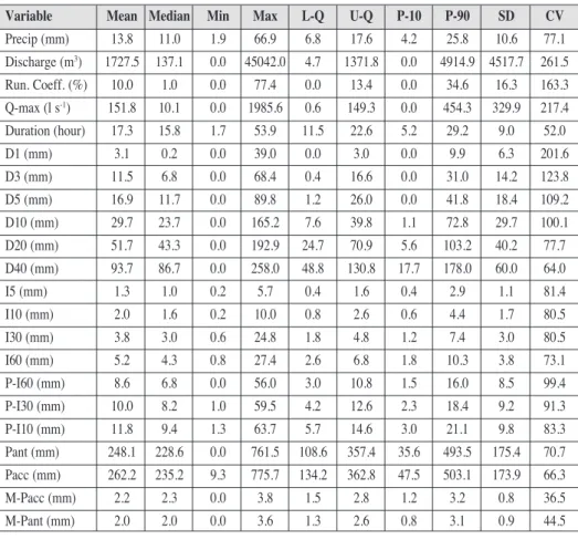
Table 2. Basic statistics of the discharge and rainfall variables for all events, n = 161.
Variable Mean Median Min Max L-Q U-Q P-10 P-90 SD CV
Precip (mm) 13.8 11.0 1.9 66.9 6.8 17.6 4.2 25.8 10.6 77.1
Discharge (m3) 1727.5 137.1 0.0 45042.0 4.7 1371.8 0.0 4914.9 4517.7 261.5
Run. Coeff. (%) 10.0 1.0 0.0 77.4 0.0 13.4 0.0 34.6 16.3 163.3
Q-max (l s-1) 151.8 10.1 0.0 1985.6 0.6 149.3 0.0 454.3 329.9 217.4
Duration (hour) 17.3 15.8 1.7 53.9 11.5 22.6 5.2 29.2 9.0 52.0
D1 (mm) 3.1 0.2 0.0 39.0 0.0 3.0 0.0 9.9 6.3 201.6
D3 (mm) 11.5 6.8 0.0 68.4 0.4 16.6 0.0 31.0 14.2 123.8
D5 (mm) 16.9 11.7 0.0 89.8 1.2 26.0 0.0 41.8 18.4 109.2
D10 (mm) 29.7 23.7 0.0 165.2 7.6 39.8 1.1 72.8 29.7 100.1
D20 (mm) 51.7 43.3 0.0 192.9 24.7 70.9 5.6 103.2 40.2 77.7
D40 (mm) 93.7 86.7 0.0 258.0 48.8 130.8 17.7 178.0 60.0 64.0
I5 (mm) 1.3 1.0 0.2 5.7 0.4 1.6 0.4 2.9 1.1 81.4
I10 (mm) 2.0 1.6 0.2 10.0 0.8 2.6 0.6 4.4 1.7 80.5
I30 (mm) 3.8 3.0 0.6 24.8 1.8 4.8 1.2 7.4 3.0 80.5
I60 (mm) 5.2 4.3 0.8 27.4 2.6 6.8 1.8 10.3 3.8 73.1
P-I60 (mm) 8.6 6.8 0.0 56.0 3.0 10.8 1.5 16.0 8.5 99.4
P-I30 (mm) 10.0 8.2 1.0 59.5 4.2 12.6 2.3 18.4 9.2 91.3
P-I10 (mm) 11.8 9.4 1.3 63.7 5.7 14.6 3.0 21.1 9.8 83.3
Pant (mm) 248.1 228.6 0.0 761.5 108.6 357.4 35.6 493.5 175.4 70.7
Pacc (mm) 262.2 235.2 9.3 775.7 134.2 362.8 47.5 503.1 173.9 66.3
M-Pacc (mm) 2.2 2.3 0.0 3.8 1.5 2.8 1.2 3.2 0.8 36.5
M-Pant (mm) 2.0 2.0 0.0 3.6 1.3 2.6 0.8 3.1 0.9 44.5
1. Given a catchment size of 0.995 km2a value of 1 m3corresponds to 1.005 m3km-2or 0.001 mm. Therefore discharge
Median event rainfall amounted to 11.0 mm, with lower and upper quartiles of 6.8 and 17.6 mm, respectively. Ten percent of the sample registered more than 25.8 mm. Most rainfall events were of large duration with a median of almost 16 hours and 50% of the events having a duration between 11.5 and 22.6 hours. With respect to rainfall intensities, maximum 5-minute amounts had a median of 1.0 mm and 25% of the events registered more than 1.6 mm (19.2 mm h-1). Maximum 60-minute intensity ranged
between 0.8 mm and 27.4 mm, with 10% of the sample in excess of 10.3 mm. Regarding antecedent rainfall conditions (Pant) the median was 228.6 mm, being the lower and upper quartiles 108.6 mm and 357.4 mm, respectively. Table 2 also includes the statistical descriptors for other variables used as indicators for antecedent catchment conditions.
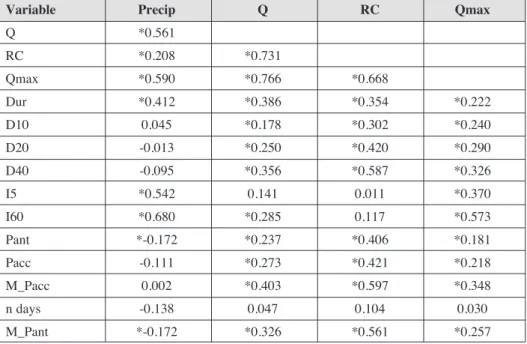
Linear regression analysis between discharge and the rainfall variables were carried out (Table 3). Although the relation between event rainfall and discharge is significant the coefficient of correlation R is low. Similarly, but with even lower R-values, discharge correlates significantly with mean accumulated rainfall (M_Paccum), event duration and the amount of rainfall registered during 40 days prior to the event (D40), citing only the variables with greater R (Table 3). The runoff coefficient showed best correlations with variables indicating antecedent moisture conditions, the coefficient R is low for rainfall and is not significant in the case of rainfall intensities (Table 3).
Table 3. Correlation coefficients between selected event characteristics (*significant at p < 0.05, n=161). Names of variables are explained in the text.
Variable Precip Q RC Qmax
Q *0.561
RC *0.208 *0.731
Qmax *0.590 *0.766 *0.668
Dur *0.412 *0.386 *0.354 *0.222
D10 0.045 *0.178 *0.302 *0.240
D20 -0.013 *0.250 *0.420 *0.290
D40 -0.095 *0.356 *0.587 *0.326
I5 *0.542 0.141 0.011 *0.370
I60 *0.680 *0.285 0.117 *0.573
Pant *-0.172 *0.237 *0.406 *0.181
Pacc -0.111 *0.273 *0.421 *0.218
M_Pacc 0.002 *0.403 *0.597 *0.348
n days -0.138 0.047 0.104 0.030
M_Pant *-0.172 *0.326 *0.561 *0.257
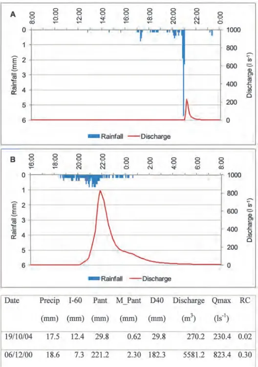
Figure 2. Two examples of flood hydrographs, produced under dry (A) and humid (B) antecedent moisture conditions. Characteristics of rainfall and discharge
moisture conditions. In this sense, Fig. 2 compares two flood hydrographs produced during the 19/10/2004 and the 6/12/2000. Although the first event registered higher maximum rainfall intensity (69.6 mm h-1) as compared to the second one with 9.6 mm h-1,
the latter produced much higher discharge with 5581 m3 as opposed to 270 m3.
Accumulated antecedent rainfall was approximately 30 mm in the first case, with a mean daily value of 0.62 mm. These values contrast with Pant of 221 mm and M_Pant of 2.30 mm. Peak discharge was also higher with humid catchment conditions. A great difference is also observed with respect to the runoff coefficient, being approximately 15 times higher in the humid case (Fig. 2).
In conclusion, the regression analysis, as well as the comparison of hydrographs indicates the importance of antecedent rainfall conditions. In order to investigate the importance of antecedent soil moisture conditions in depth, the next step is to analyze the relationship between soil water content in the valley bottom and its relations with rainfall and discharge.
4.2. The role of soil moisture
The spatial variation of water content on soils of the valley bottom, i.e. the differences between probes belonging to the same depth, was described in Maneta et al. (2008), demonstrating that soil moisture close to the surface was less variable probably because they are wetted and dried by evaporation and transpiration more homoge-neously than soils at lower depths. There, the effect of soil heterogeneities is presumably stronger in the redistribution of water within the soil and plant water extraction is more heterogeneous. The amplitude of the standard deviation of soil moisture increases with depth and is highest at 0.7 and 0.9 m from the soil surface.
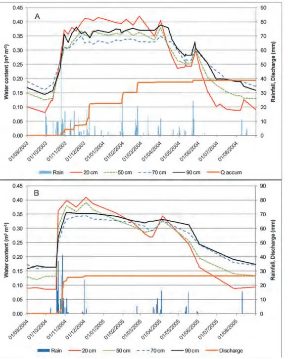
Fig. 3 shows average soil moisture at each depth for the hydrological years 2003 and 2004, together with daily rainfall and accumulated discharge. All depths experienced a sharp increase of water content in autumn and a less steep decrease corresponding to the drying phase in spring. The decrease is less pronounced for the probes at greater depths. As expected, temporal variation is highest close to the surface (0.2 m). During the summer months, from July to September, water content in the upper surface layer drops to 0.08 m3m-3and reaches 0.42 m3m-3during humid periods. The
probes installed at greater depth (0.7 and 0.9 m) showed a similar behaviour, with moisture values during summer of approximately 0.17 m3 m-3. The probes at 70 cm
registered, however, lower maximum values (0.35 m3m-3) as compared to the deepest
probes, probably related with their lower porosity and lower field capacity (Table 1), indicating lower values at saturation but also a faster drainage.
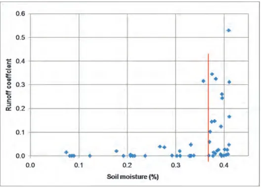
No discharge was generally observed during summer, except for low frequency thunderstorms (> 1 year). The strong increase of discharge in autumn was always related with high soil moisture content, generally above 0.30 m3 m-3 (Fig. 3). Regression
threshold can be observed at a water content of 0.37 m3m-3. Below this value runoff
coefficients do not exceed 0.05 and above this value events with high runoff coefficients were registered. This threshold behaviour in runoff production also explains the bad correlation between rainfall and runoff. With 150 mm of antecedent rain and mean accumulated precipitation (M_Paccum) ≥ 2.0 mm soil moisture reaches 0.37 m3m-3. This
dichotomous behaviour was used to group the event discharges. All events exceeding both values were classified as Humid. Initially all events lower than these values were classified as Dry, but rainfall-runoff regression analysis did not produce satisfying results. A further group (Intermediate) was established with Paccum > 150 mm and M_Paccum
in the range of 1.5 – 2.0 mm. Except for one case, all events occurred during spring, representing the drying phase but with relatively high antecedent rainfall.
4.3. Empirical rainfall-runoff modeling
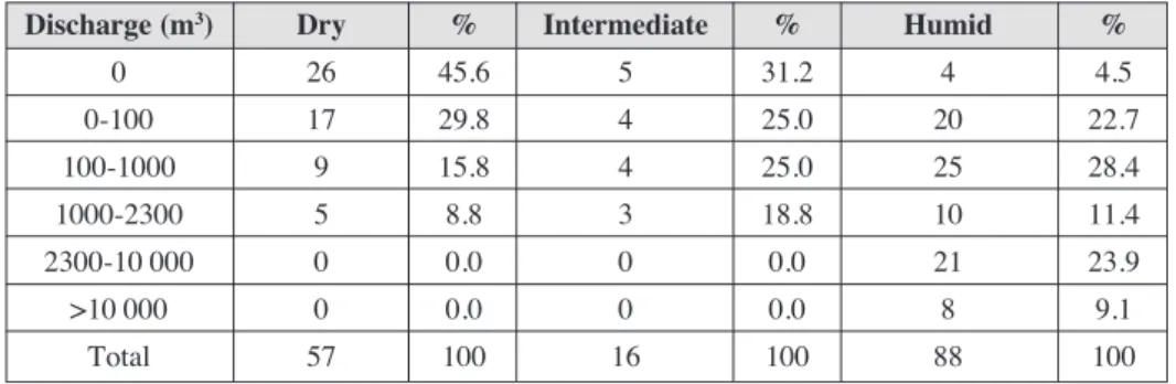
The non-parametric ANOVA Kruskal-Wallis test showed that grouping of discharge is highly significant with p < 0.0000. Group Humid is significantly different from groups Dry and Intermediate, though the Dry events are not significantly different from the intermediate ones. Table 4 shows the frequency distribution of discharge for the three groups. With dry antecedent conditions approximately 45% of the events did not generate
discharge, whereas this percentage drops to 4% in the case of the humid events. This large difference is also reflected by the maximum runoff value, with 2227 and 45 042 m3, for
the dry and the humid case, respectively. Taking the maximum dry event for class separation (2300 m3), a total of 29 humid events exceeded this amount (Table 4). The
Intermediate events did not exceed 2300 m3.
Table 4. Frequency of discharge amounts grouped by antecedent rainfall conditions.
Discharge (m3) Dry % Intermediate % Humid %
0 26 45.6 5 31.2 4 4.5
0-100 17 29.8 4 25.0 20 22.7
100-1000 9 15.8 4 25.0 25 28.4
1000-2300 5 8.8 3 18.8 10 11.4
2300-10 000 0 0.0 0 0.0 21 23.9
>10 000 0 0.0 0 0.0 8 9.1
Total 57 100 16 100 88 100
These differences are also reflected by the runoff coefficients, with a mean value of 0.17 and 0.01 for the humid and dry cases, respectively (Table 5). Also peak discharges were significantly higher with humid antecedent moisture conditions. These differences are not related with the maximum intensities or the amount of the rainfall events, being even higher in the case of the dry events (Table 5). The Dry group, for example, registered median 5-minute maximum rainfall of 1.2 mm as compared to 0.8 mm for the humid cases. This means that even with on average lower event rainfall amounts and intensities under humid antecedent catchment conditions runoff production was clearly higher.
Although the Intermediate events correspond to a group with a small sample size and discharge is not significantly different from the Dry group, under similar rainfall event they generated higher runoff. Except for one case, all these events occurred in spring (between March and April), during the drying phase of the catchment, i.e. antecedent rainfall was high, but with relatively low amounts immediately prior to the events.
Table 5. Comparison of event characteristics grouped by antecedent rainfall conditions (names of variables and grouping criteria are explained in the text).
Ant. cond. Humid Dry Humid Dry Interm. Humid Dry Humid Dry
Variable Mean Mean Median Median Median LQ LQ UQ UQ
Precip 12.9 15.8 10.6 11.6 10.3 5.0 8.3 16.0 18.4
Discharge 2952.3 192.7 640.4 4.0 94.4 60.9 0.0 3614.5 65.2
RC 0.17 0.01 0.11 0.00 0.01 0.01 0.00 0.30 0.00
Qmax 237.5 40.8 32.3 0.7 23.7 4.3 0.0 300.6 15.0
Duration 20.6 13.8 18.7 12.7 11.8 14.3 6.6 25.7 19.2
D1 2.9 3.5 0.4 0.1 0.3 0.0 0.0 1.8 5.0
D3 12.7 9.8 8.1 2.6 5.3 1.7 0.0 16.6 16.0
D10 36.9 19.7 27.7 15.4 21.2 15.2 1.5 48.4 31.2
D40 128.1 45.4 128.3 39.8 85.6 86.0 18.4 166.3 67.1
I5 1.1 1.6 0.8 1.2 1.0 0.4 0.8 1.4 2.4
I10 1.8 2.5 1.3 2.0 1.6 0.8 1.2 2.0 3.6
I30 3.4 4.4 2.5 3.6 3.1 1.5 2.4 4.4 7.0
I60 4.8 6.0 3.5 5.2 4.3 2.3 3.2 5.9 8.4
P-I60 8.1 9.7 6.8 7.4 5.1 2.1 4.1 10.1 11.9
Pant 342.4 86.7 310.1 69.9 303.9 212.7 29.8 460.4 127.7
Pacc 355.3 102.4 319.7 82.0 313.5 228.2 42.4 472.8 138.2
M_Pacc 2.8 1.4 2.7 1.4 1.6 2.5 1.1 2.9 1.8
n days 127.5 76.0 118.0 51.0 200.0 86.0 46.0 170.5 77.0
M_Pant 2.7 1.1 2.6 1.2 1.5 2.4 0.6 2.8 1.4
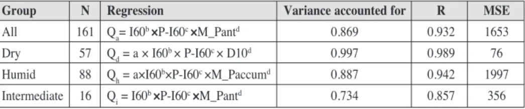
The best results were obtained using maximum 60-minute rainfall (I60) and the event rainfall subtracting I60 (P-I60), together with a variable reflecting the antecedent rainfall conditions for the complete dataset, as well as the grouped data. Table 6 presents the regression equations together with the variance accounted for by the model, the correlation coefficient R and the mean squared error (MSE) for the complete dataset and the grouped data and table 7 includes the constants (exponents of the equations) and their p-level.
Table 6. Summary of regression results. All regressions are significant at p < 0.0001.
Group N Regression Variance accounted for R MSE
All 161 Qa= I60b ×P-I60c ×M_Pantd 0.869 0.932 1653
Dry 57 Qd= a × I60b × P-I60c × D10d 0.997 0.989 76
Humid 88 Qh= a×I60b×P-I60c ×M_Paccumd 0.887 0.942 1997
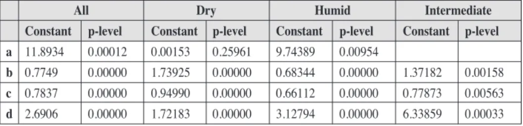
Table 7. Values of the constants and their p-level for the different regression equations.
All Dry Humid Intermediate
Constant p-level Constant p-level Constant p-level Constant p-level
a 11.8934 0.00012 0.00153 0.25961 9.74389 0.00954
b 0.7749 0.00000 1.73925 0.00000 0.68344 0.00000 1.37182 0.00158
c 0.7837 0.00000 0.94990 0.00000 0.66112 0.00000 0.77873 0.00563
d 2.6906 0.00000 1.72183 0.00000 3.12794 0.00000 6.33859 0.00033
In the case of the complete dataset the best regression accounted for 0.87 of the data variance with a mean squared error (MSE) of 1653 m3. Higher correlation coefficients
were obtained grouping the data. In the case of the Dry group the relationship improved, when including rainfall fallen 10 days prior to the event (D10) accounting for 0.997 of the variance and a MSE of 76 m3.
For the Humid group the best results were obtained using mean accumulated precipitation (M_Paccum), explaining 0.887 of the sample variance. Mean antecedent rainfall (M_Pant) yielded better results for the complete dataset and the Intermediate events. Figs. 5 and 6 present the predicted vs. the observed values for the Dry and the Humid cases, respectively, showing a linear distribution. The residuals produced by the empirical models yielded normal frequency distributions. These two aspects of the regression results, indicates, apart from the high regression coefficients, the quality of the modelling results.
Although similar variables explain discharge production, the exponents vary (Table 7). For example, rainfall intensity (I60) is more important in the dry events than in the humid ones, with an exponent of 1.74 and 0.68, respectively. Although the results show that discharge in all cases depends on the amount and intensity of rainfall, as well as the antecedent rainfall, different event rainfall thresholds can be established, being 2 mm, 8 mm and 12 mm for the Humid, Intermediate and Dry groups, respectively.
The regression equations were used to estimate missing discharge data. For the complete dataset the estimated discharge accounted for 11.4% of the total observed amount. The estimated values were used for completing the annual and monthly runoff amounts.
4.4. Long-term rainfall variation
Figure 5. Observed vs. predicted discharge of the dry events.
less than 60% of mean precipitation. It finishes when monthly rainfall exceeds 100% of the average. However, the application of this method shows certain limitations. During the summer dry period (from June to September) the occurrence of two consecutive months with less than 60% rainfall is common. Zero rainfall in July or August is frequent, however this value constitutes less than 60% of the mean. On the other hand, one high intensity event produces a monthly amount that surpasses the average value in summer, but this cannot be considered as the end of a drought because it neither affects plant growth, nor does it produce significant amounts of runoff. Furthermore, prolonged dry periods were in some cases interrupted by a month with high rainfall. In this case, that month is included in the drought. The present study does not aim to make general statements about droughts in the study region, but intends to improve understanding of the relationship between rainfall and runoff production. The analysis was carried out in order to be able to interpret the runoff data in a long-term context. Table 8 presents the result of the analysis based on the departures from mean monthly rainfall. A dry period commences when two consecutive months register below 60% of the mean rainfall. Their end is defined when the negative trend clearly finished; this means that short interruptions (one or two months) of above-average rainfall are not considered to constitute the end of the dry period. Considering only periods with a deficit in excess of -200 mm (Table 8), the duration of droughts varied between 6 and 45 months, with deficits ranging from -203 to -605 mm. Using these criteria, 37% of the 105 years were droughts with a mean deficit of -387 mm and an average duration of approximately two years.
Table 8. Dry periods in Cáceres, their duration and total water deficit (Deficit). The annual and monthly deficits are an expression of the drought intensity.
Drought Start End Duration Deficit Annual Monthly
(month) (mm) Deficit (mm) Deficit (mm)
D1 Feb 1908 Sep 1910 21 367.5 210.0 17.5
D2 Jul 1917 Dec 1917 6 213.4 426.8 35.6
D3 May 1919 Jan 1923 45 536.3 143.0 11.9
D4 Aug 1930 Oct 1935 63 603.4 114.9 9.6
D5 Oct 1943 Oct 1945 25 445.4 213.8 17.8
D6 Jun 1948 Nov 1950 30 430.9 172.4 14.4
D7 Oct 1952 Oct 1954 25 548.4 263.2 21.9
D8 Nov 1956 Nov 1958 25 492.1 236.2 19.7
D9 Apr 1964 Aug 1965 17 268.1 189.2 15.8
D10 Jul 1966 Dec 1968 30 266.7 106.7 8.9
D11 Feb 1970 Dec 1971 23 377.7 197.1 16.4
D12 Aug 1973 Mar 1976 32 503.6 188.9 15.7
D13 Jan 1980 Mar 1983 39 604.8 186.1 15.5
D14 Aug 1988 Mar 1989 8 221.8 332.7 27.7
D15 Apr 1991 Mar 1993 24 376.4 188.2 15.7
D16 Dec 1994 Oct 1995 11 202.9 221.3 18.4
D17 Nov 2004 Sep 2005 11 342.5 373.6 31.1
D18 Sep 2008 Nov 2009 15 266.4 213.1 17.8
D19 Jun 2011 Aug 2012 15 291.4 233.1 19.4
Mean 24.5 387.4 189.9 15.8
From Fig. 7 it can also be depicted that prolonged periods occur when several droughts take place consecutively, i.e. with little time in between. The most extreme period commenced in 1943 and lasted until 1958 with 4 consecutive droughts. More recently, between 1991 and 1994, two successive droughts took place (Table 8). In contrast, the last decade has been more variable with moderate droughts interrupted by periods with above average rainfall. The data do not indicate any trend in increasing drought frequency or intensity.
Exceptionally humid periods can also be recognized in Fig. 7. They are less frequent, but were responsible of very large amounts of rainfall. For example, between 11/1995 and 12/1997 (26 months) rainfall exceeded in 873 mm the average total rainfall for this period.
the three droughts mentioned in table 8. Both catchments have a very similar rainfall-runoff response (analysis not presented here). The study period belonging to Guadalperalón consisted of 3 dry years and 2 very humid years, whereas the Parapuños data also include two years with average annual rainfall (Table 9).
Additionally to the 3 drought periods, the year 2001, although not considered a prolonged dry period, registered low precipitation (378.7 mm). Separating these periods from the rest which registered normal and above average rainfall, reveals a great difference between the two groups (Table 10). During a total of 58 months the dry periods with 1370 mm of rainfall produced only 11.8 mm of discharge, representing a
runoff coefficient (RC) of 0.009. In contrast, during the normal and humid periods (95 months) with 4571 mm of rainfall, discharge amounted to 506 mm (RC = 0.11). Monthly discharge on average was 0.20 mm during the dry periods and 5.33 mm during the normal to humid periods, i.e. approximately 27 times higher.
Table 9. Annual values of rainfall, discharge, runoff coefficient and runoff deficit of the Guadalperalón (1991-996) and Parapuños (2000-2006) catchments.
Year Rainfall (mm) Discharge (mm) Runoff coefficient Runoff deficit (mm)
1991-92 386.3 3.9 0.010 382.4
1992-93 372.8 4.9 0.013 367.9
1994-95 330.6 7.5 0.023 323.1
1995-96 720.1 102.3 0.142 617.8
1996-97 723.4 127.1 0.176 596.3
2000-01 801.8 187.7 0.234 614.1
2001-02 378.7 4.4 0.012 374.3
2002-03 580.4 74.0 0.128 506.4
2003-04 526.4 38.8 0.074 487.6
2004-05 336.3 26.6 0.079 309.7
2005-06 395.4 25.1 0.063 370.3
2006-07 648.2 76.0 0.117 572.2
Mean 517.4 56.5 0.109 460.9
Table 10. Rainfall, discharge and runoff coefficients grouped according to dry and normal or humid periods.
Catchment Class Rainfall (mm) Runoff (mm) Runoff coefficient
Guadal Drought 15 640.4 4.7 0.007
Drought 16 203.3 5.6 0.028
Normal/humid 1421.9 229.4 0.161
Parap Normal/humid 2102.1 323.4 0.154
Dryyear 378.7 4.4 0.012
Normal/humid 1046.9 101.1 0.097
Drought 17 147.7 3.7 0.025
TOTAL Droughts 1370.1 11.8 0.009
Normal/humid 4571.0 506.1 0.111
A more homogenous distribution of rainfall along the hydrological year resulted in low discharge, as compared to a year when most rainfall was concentrated during few months. Examples are the years 2004 and 2003, the former was dry but rainfall was more concentrated, whereas the latter was normal with a more homogenous rainfall
distribution (Fig. 8). As a consequence, runoff coefficients were similar and annual discharge of the drier year 2004 was only little less than 2003 (Table 9).
The irregularity of rainfall, especially the occurrence of dry and humid periods, in combination with knowledge about the hydrological processes gained in more specific studies at the event scale, including soil moisture and groundwater movement, explain the variation of monthly discharge production. In contrast, mean monthly rainfall and runoff values are interesting, for that they illustrate on the average seasonality. In our study area discharge was almost zero from June to September (Fig. 10). Although October was the month with the highest mean rainfall, it produced fairly low runoff. After the summer dry period, a considerable amount of rain (170 mm) was necessary for generating large amounts of discharge. Therefore mean runoff was highest in December and January. Rainfall decreased from February onwards and most of the time soil moisture in the valley bottom stayed below the threshold value, defined in the Parapuños catchment at 0.37 m3m-3at 0.2 m depth. The mean annual rainfall distribution during
the 12-year study period is slightly different from the large series (Fig. 10), with higher precipitation in October and slightly lower rainfall in winter and spring.
5. Discussion
Gallart et al. (2008) comparing seven Mediterranean catchments of varying size stated that most of them showed a wet season when precipitation exceeded potential evapotranspiration, presenting saturation excess runoff generation mechanisms and
relevant baseflow contribution. Infiltration excess (Hortonian) overland flow existed during summer storms in some catchments. These findings coincide with ours in that “wet” mechanisms are the most important. It is, however, very difficult to compare the dehesa catchments with others in the Mediterranean. Many of the study basins are located in mountainous areas and have thus higher annual rainfall and lower potential evapotranspiration (e.g. Gallart et al., 2005; García-Ruiz et al., 2008). Also lithology, vegetation and topography are important factors.
Regarding climate and vegetation, research carried out in California oak woodlands (Dahlgren et al., 2001) permits comparison. The water dynamics are however slightly different. In the case of California, Hortonian overland flow was rarely observed and annual discharge and runoff coefficients were higher than in the Extremadura catchments (Dahlgren et al., 2001). These differences may be explained by the annual rainfall total (higher) and soil properties (greater depth) (Schnabel et al., in press). In California large amounts of runoff are generated due to saturation of the upper soil layer as a consequence of a nearly impervious clay horizon (Swarovski et al., 2011). In contrast, the Spanish catchments generate Hortonian overland flow during high intensity storms. Common to both areas is that saturation excess and preferential flow are responsible for most of the total runoff, being the threshold for saturation lower in Extremadura as compared to the Californian catchment. Variability of discharge was also higher in our catchments.
6. Conclusions
Regression analysis as well as the comparison of hydrographs illustrate on the importance of antecedent rainfall conditions. Soil moisture in the valley bottom was crucial to understand the hydrological behaviour of the catchment. A soil moisture threshold of 0.37 m3m-3was defined above which runoff coefficients increase sharply.
This situation is reached with 170 mm of antecedent rain falling in a continuous way. These results coincide with findings of previous studies carried out in the study area, suggesting that saturation excess flow and preferential subsurface flow are important processes. Hortonian type overland flow is thought to dominate under dry conditions and rainfall of high intensity.
The relationship between rainfall, soil moisture and runoff permitted grouping of the event-scale database. Non-linear regression analysis was carried out for the complete data set and the groups. Highly significant regression models were obtained which explained event discharge using three variables: Maximum 60-minute rainfall intensity, the event rainfall deducting I60 and a variable that expresses antecedent rainfall conditions. Grouping of the events improved the results.
Acknowledgements
Research was financed by the Spanish Ministry of Education and Science through projects REN2001-2268-C02, CGL2004-04919-C02-02, CGL2008-01215, CGL2011-23361.
References
Beven, K. 2002. Runoff generation in semi-arid areas. In Dryland Rivers: Hydrology and Geomorphology of Semi-Arid Channels, L.J. Bull, M.J. Kirkby (eds.), John Wiley and Sons, New York, pp. 57-105.
Bos, M.G., Replogle, J.A., Clemmens, A.J. 1986. Aforadores de caudal para canales abiertos. Vol. 38.International Institute for Land Reclamation and Improvement, Wageningen, The Netherlands.
Castillo, V.M., Gómez-Plaza, A., Martínez-Mena, M. 2003. The role of antecedent soil water content in the runoff response of semiarid catchments: a simulation approach. Journal of Hydrology284, 114-130.
Ceballos A., Schnabel, S. 1998. Hydrological behaviour of a small catchment in the Dehesa landuse system (Extremadura, SW Spain). Journal of Hydrology210, 146-160.
Dahlgren, R.A., Tate, K.W., Lewis, D.J., Atwill, E.R., Harper, J.M., Allen-Diaz, B.H. 2001. Watershed research examines rangeland management effects on water quality. Californian Agriculture55, 64-71.
Dirksen, C. 1999. Soil Physics Measurements. Catena Verlag, Reiskirchen, 154 pp.
Gallart, F., Llorens, P., Latron, J., Regüés, D. 2002. Hydrological processes and their seasonal controls in a small Mediterranean mountain catchment in the Pyrenees. Hydrology and Earth System Sciences6, 527-537.
Gallart, F., Latron, J. Llorens, P. 2005. Catchment dynamics in a Mediterranean mountain environment. The Vallcebre research basins (South Eastern Pyrenees) I: Hydrology. Developments in Earth Surface Processes7, 1-16.
Gallart, F., Amaxidis, Y., Botti, P., Canê, G., Castillo, V., Chapman, P., Froebrich, J., García-Pintado, J., Latron, J., Llorens, P., Lo Porto, A., Morais, M., Neves, R., Ninov, P., Perrin, J.L., Ribarova, I., Skoulikidis, N., Tournoud, M.G. 2008. Investigating hydrological regimes and processes in a set of catchments with temporary waters in Mediterranean Europe. Hydrological Sciences Journal 53, 618-628.
García-Ruiz, J.M., Arnáez, J., Beguería, S., Seeger, M., Martí, C., Regüés, D., Lana-Renault, N., White, S. 2005. Flood generation in an intensively disturbed, abandoned farmland catchment, Central Spanish Pyrenees. Catena59, 79-92.
García-Ruiz, J.M., Regüés, D., Alvera, B., Lana-Renault, N., Serrano-Muela, P., Nadal-Romero, E., Navas, A., Latron, J., Martí-Bono, C. 2008. Flood generation and sediment transport in experimental catchments along a plant cover gradient in the Central Pyrenees. Journal of Hydrology356, 245-260.
Gómez Amelia, D. 1985. La penillanura cacereña. Estudio geomorfológico. Universidad de Extremadura, Cáceres.
Lana-Renault, N., Latron, J., Regüés, D. 2007. Streamflow response and water-table dynamics in a sub-Mediterranean research catchment (Central Pyrenees). Journal of Hydrology347, 497-507. Latron, J., Gallart, F. 2008. Runoff generation processes in a small Mediterranean research
Latron, J., Soler, M., Llorens, P., Gallart. F. 2008. Spatial and temporal variability of the hydrological response in a small Mediterranean research catchment (Vallcebre, Eastern Pyrenees). Hydrological Processes22, 775-787.
Lewis, D., Singer, M.J., Dahlgren R.A., Tate, K.W. 2000. Hydrology in a California oak woodland watershed: A 17-year study. Journal of Hydrology240, 106-117.
Maneta, M. 2006. Modeling of the hydrologic processes in a small semiarid catchment. Unpublished PhD Thesis, Universidad de Extremadura, Cáceres, 310 pp.
Maneta M.P., Schnabel, S., Jetten V.G. 2007. Continuous spatially distributed simulation of surface and subsurface hydrological processes in a small semi-arid catchment. Hydrological Processes 21,2196-2214.
Maneta, M., Pasternack, G.B., Wallender, W.W., Jetten, V.D., Schnabel, S. 2007. Temporal instability of parameters in an event-based distributed hydrologic model applied to a small semi-arid catchment. Journal of Hydrology341, 207-221.
Maneta, M., Schnabel, S., Wallender, W., Panday, S., Jetten, V. 2008. Calibration of an evapotranspiration model to simulate soil water dynamics in a semiarid rangeland. Hydrological Processes22, 4655-4669.
Moré, J.J. 1977. The Levenberg-Marquardt Algorithm: Implementation and Theory. In Lecture Notes in Mathematics, G.A. Watson (ed.), Springer, Berlin, pp. 106-116.
Schnabel, S. 1997. Soil erosion and runoff production in a small watershed under silvo-pastoral landuse (Dehesas) in Extremadura, Spain. Geoforma Ediciones, Logroño.
Schnabel, S., Dahlgren, R.A., Moreno, G. In press. Soil and water dynamics. In Mediterranean Oak Woodland Working Landscapes. Dehesas of Spain and Rangelands of California, P. Campos, L. Huntsinger, J.L. Oviedo, P.F. Starrs, M. Díaz, R. Standiford, G. Montero (eds.), Springer, New York.
Shaw, E.M. 1988.Hydrology in practice. Van Nostrand Reinhold, London.
Swarowsky, A., Dahlgren, R.A., Tate, K.W., Hopmans, J., O’Geen, A.T. 2011. Catchment-scale soil water dynamics in a Mediterranean oak woodland. Vadose Zone Journal10, 800-815. Van Schaik, N.L.M.B., Schnabel, S., Jetten, V.G. 2008. The influence of preferential flow on
hillslope hydrology in a semi-arid watershed (in the Spanish Dehesas). Hydrological Processes22, 3844-3855.
Van Schaik, N.L.M.B. 2009. Spatial variability of infiltration patterns related to site characteristics in a semi-arid watershed. Catena78, 36-47.