Parameter Settings for Reconstructing
Binary Matrices from Fan-beam
Projections
Antal Nagy and Attila Kuba
Department of Image Processing and Computer Graphics, University of Szeged, Hungary
The problem of reconstruction of binary matrices from their fan-beam projections is studied. A fan-beam projection model is implemented and used in systematic experiments in order to determine the optimal parameter values for data acquisition and reconstruction algorithm. The fan-beam model, the reconstruction algorithm, the simulation experiments, and the results are discussed in the paper.
Keywords: discrete tomography, fan-beam projections, simulated annealing.
1. Introduction
Discrete tomography (DT) is used for
recon-structing special objects consisting of a few types of known homogeneous materials. For example, if we know that the object is made of wood, then the space contains only two materi-als: wood and air. Such objects can be repre-sented with two-valued functions. The know-ledge of the discrete range of the function to be reconstructed can also reduce the number of necessary projections drastically. For a sum-mary of theory and applications of DT see1].
This paper deals with the reconstruction of bi-nary matrices, i.e., the matrix elements can be either 0 or 1. The reconstruction methods of binary matrices from parallel projections are available, i.e., when the sums of matrix elements along the lines parallel to given directions are given(e.g., row and column sums)is a well
un-derstood area of DT2, 3]. Surprisingly, there
are few results published in connection with fan-beam projections4, 5]. Afan-beamprojection
Detectors
Detectors
S0 Sk
Cr
q0
j
x y
(a) Using line integrals
Detectors Detectors
S0 Sk
Cr
a j
q0
y
x
(b) Using strip integrals
is a collection of sums of matrix elements ar-ranged in a fan-shaped area determined by two rays having the same source point(Fig. 1).
Most of the currently used CT scanners apply fan-beam projections. There are also other ap-plications of tomography(e.g., non-destructive
testing with X-rays 6] or neutrons 7]) where
fan-beam projections are collected. At the same time, most of the papers about DT deal with parallel projections. We believe that fan-beam projections should play similarly important role in the applications of DT as in the case of classi-cal(non-discrete)tomography. For this reason
it is important to study the problems connected with fan-beam projections in DT(the only paper
we found is8]). Such studies can be interesting
not only from the viewpoint of the implemented reconstruction algorithm (more generally, the
software), but also from the viewpoint of the
construction of the data acquisition system, i.e., the hardware of the DT.
This paper deals with the optimal setting of the geometric parameters in case of fan-beam pro-jections. The method for this study is simula-tion. A software system is implemented which is able to simulate the collection of projections of binary matrices (2D objects), then to
per-form the reconstruction, and finally, to compare the reconstructed binary matrix with the origi-nal one. Simulation is suitable for studying the effects of different parameters of a complex sys-tem separately and for giving an estimate of the performance of a similar real system. In a pre-vious work9] we used this simulation system
for studying the reconstruction algorithm. Now we investigate also the differences between the
half-line integrals(Fig. 1(a))andstrip integrals
(Fig. 1(b)) when changing the fan-beam
geo-metric parameters(e.g. changing the number of
sources and detector elements). A series of
re-constructions is performed varying only one pa-rameter while keeping all others fixed. The pro-jections are computed analytically, according to the actual parameter setting. The measurement errors are simulated by additive random noise. As reconstruction algorithm a version of the ran-dom search optimization method of Simulated Annealing (SA) was implemented 10]. The
reconstructed images were compared with the original image on the basis of the relative mean square error11, 12].
The structure of the papers is as follows. In Sec-tion 2 the reconstrucSec-tion problem is introduced with the necessary definitions and notation in the case of fan-beam projections. In Section 3 the DT reconstruction problem is reformulated as an optimization problem, which is solved by the method of SA. The results of our ex-periments and our discussions are detailed in Section 4. Finally, the last chapter gives the conclusions we obtained from our works.
2. The Reconstruction Problem and Fan-beam Projections
Let f be an integrable real function on theR
2
plane. LetSbe a point, calledsource point, and
vθ be a unit vector in the directionθ 2 0 2π)
on the plane. Consider the integrals of f along the half-lines starting fromSin directionvθ:
Rf](S θ)= 1 Z
0
f(S+uvθ)du: (1)
The transformation defined by(1)is called the
fan-beam projection of f taken from the point S in the direction θ. Given a set S of source
points, the reconstruction problem using fan-beam projectionscan be posed as follows.
RECONSTRUCTIONFB(S)
Given: An integrable function,
g:S0 2π)!R.
Task: Construct a function f such that
Rf](S θ) = g(S θ) (2)
for all S 2 S for almost every
θ 20 2π).
In this paper we are interested in the reconstruc-tion of special funcreconstruc-tions from fan-beam projec-tions. Henceforth, let us suppose that the sup-port of f can be covered by a n n regular
latticeW such that f is constant on each 11
square of the lattice, namelyfcan take the value of either 0 or 1. That is, f can be represented by a nn binary matrix or, equivalently, by a
vectorx 2f0 1g
J wherex
j denotes thejth
ele-ment of the matrix, say, in a row by row order
j=1 2 ::: JandJ=n
2.
integrals are taken not along half-lines but on areas(let us call themfans)determined by two
half-lines having angleα between them. LetSk, k = 1 2 ::: K, denote the number of
source points. They are situated along a cir-cle Cr = f(x y)jx
2
+ y
2
= r
2
g around the
origin O, where r > 0 is large enough so
that W is in Cr. Furthermore, it is also usual
that source points are distributed alongCr
uni-formly, that is,Sk =(rcosθk rsinθk), where
θk =θ0+(k;1)2π=Kfor allk =1 2 ::: K.
Thestart angleθ020 2π)determines not only
the position of the first, but of all source points. For example, the start angleθ0 =0 means that
the first source is in the intersection of circleCr
and the positive part of axisx. The reason for the inclusion of the initial angleθ0 into the model is that since we usually have only a few(e.g.,
2–4)source points, not only their number, but
also their positions can have strong influence on the reconstruction, as we show later.
It is supposed that the integrals of the binary ma-trix are measured on a finite, say,Lnumber ofα
angle fans from each source point(Fig. 1). Fans
are created in the same way from each source
point. Fans from point Sk are distributed
uni-formly between the half-lines starting form Sk
and touching the circle containing W. The an-gle between these two tangents is denoted byϕ
(see Fig. 1). Therefore, all fans are determined
uniquely by the parametersr,L, andα.
Theith fan-beam projection samplebi, fromSk
can be described by the linear equation
J X
j=1
aijxj = bi i=1 2 ::: I (3)
whereaijdenotes the common area between the
ith fan and thejth unit square ofWandI=KL.
The elements of matrix A = (aij)I
J can be
computed knowing the positions of the squares inWand the fans starting from the source points. The specialty of(3)is that the unknown vectorx
is binary, i.e.,xj 2f0 1gfor allj=1 2 ::: J.
In our model, the fan-beam integrals are mea-sured byLdetectors placed opposite the sources uniformly along an arc having its center point in
Sk (Fig. 1). The arc of detectors is big enough
i i+1
aij
ai+1j
j
(a) Line integrals
i i+1
j
aij
ai+1j
(b) Strip integrals
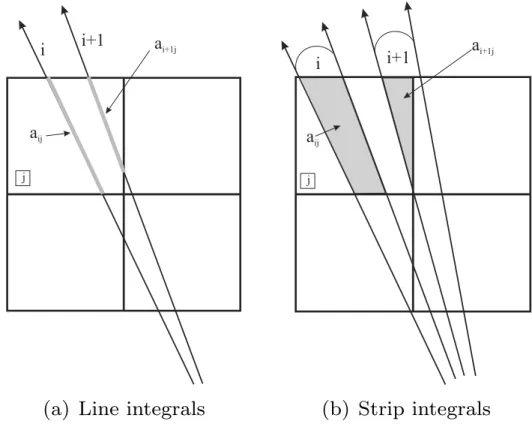
Fig. 2.Calculating the weights in the case of line and strip integrals. The grayaijis the weight of thejth unit square
for theith fan. Equally, the grayai+1jis the weigth of thejth unit square for the
such that the whole image is between the half-lines drawn from the source to the endpoints of the detector arc. Each detector measures one projection value. For simplicity, we assume that the center of the rectangleW is in the originO
of the coordinate system(Fig. 1).
The projection values are calculated in differ-ent ways in case of Eq. (3) for line and strip
integrals:
in the case of line integrals, the weights are
given by the length of the section of the
ith half-lines and the jth unit square of W
(Fig. 2(a)),
in the case of strip integrals, the weights are
given by the area of the section of the ith beam and thejth unit square ofW(Fig. 2(b)).
In real situations the projections are usually measured with a certain error. For this reason, Gaussian noise can be generated and added to the exact (analytically computed) projections
for creating noisy projection data.
In our fan-beam model the following parameters can be varied.
r: radius of circleCr, i. e. the distance of the
source points from the originO;
θ0: start angle determining the position of the first source point;
K: number of source points;
L: number of detector elements or, equiva-lently, the number of measurements from one source point;
α: fan angle;
η: percentage of the additive Gaussian noise in the projections.
3. Reconstruction by Optimization
In order to solve the reconstruction problem FB in our fan-beam model we have to find a solu-tion of the linear equasolu-tion system
Ax = b (4)
such thatxis binary. Since the number of pro-jections is usually much smaller than the num-ber of unknowns and the projections are known
with some measurement error, it is more promis-ing to try to find a binaryx, that satisfies(4)at
least about.
Equation (4) can be reformulated as an
opti-mization problem. Formally, find the minimum of the objective function
C(x)=jjAx;bjj+γ Φ(x) (5)
such thatxis binary andΦ(x)is the
regulariza-tion term withγ regularization parameter. The regularization parameter is to weight the two terms in C. In the experiments we used a spe-cial kind of function forΦproto(x), namely
Φ(x)=Φproto(x)= nm;1
X
j=0
poz(fj; f (0) j ) (6)
where poz denotes the positive part ofy. For-mally,
poz(y)=
y, ify >0
0, otherwise, (7)
and f(0)
j is a so-calledprototype function. The
prototype function is Fig. 4(b)for the Fig. 4(a)
software phantom. As optimization method, we selected the Simulated Annealing(SA)10].
3.1. Simulated Annealing
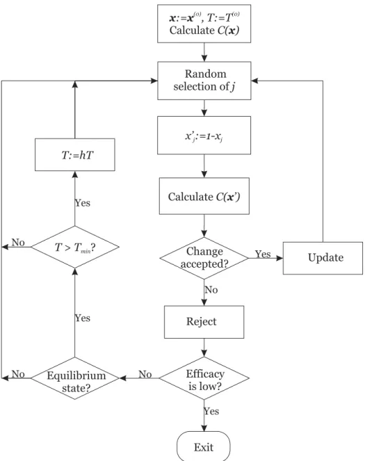
The SA method was implemented in the follow-ing way. (Fig. 3.)
The algorithm starts from an arbitrary initial bi-nary image x(0), an initial
(high) temperature
T(0) and calculates the objective function value
C(x). Then a positionjis chosen in the imagex
randomly. Letx0be the image that differs from x only by changing the value of x in position
j to the other binary value, i.e., x0
j = 1 ;xj.
This change is accepted, i.e. x is replaced by x0ifC
(x 0
) <C(x). Even if the objective
func-tion does not get smaller, the change is accepted with a probability depending on the difference
ΔC = C(x
0
);C(x). Formally, the change is
accepted even in this case if
exp(;ΔC=κT)>z (8)
where κ, T and z are, respectively, the Boltz-mann constant (11:3805 10
;23
), the current
x x:= , T:=T(0) (0)
CalculateC( )x
Reject x’ :=1-xj j
Random selection ofj
Update Change
accepted?
Efficacy is low? Equilibrium
state? T:=hT
T > Tmin?
Exit CalculateC( ’)x
Yes
Yes Yes
Yes
No No
No No
Fig. 3.Flow-chart of the implemented SA algorithm.
from the uniform distribution on the interval
0 1]. Otherwise, the change is rejected, i.e.x
is not changed in this iteration step.
If a change is rejected, the level ofefficacy of changes in the image in the last iterations is tested by counting the number of rejections in the lastNiteriterations. If this number is greater
than a given threshold value Rthr, then the SA
terminates. The temperature value is reduced if there are only very minor modifications in the value of the objective functionC(x) in the
last iterations. This is measured as the variance of the cost function in the last Nvar iterations. Equilibrium stateis reached if the estimate of
the currentΔC variance is greater than the pre-vious variance estimate.
If the equilibrium state is reached, the temper-atureT is reduced(allowing changes when the
value of the objective function is greater with smaller probabilities)and the algorithm
contin-ues with the lower temperature value(T is
re-placed byhT, wherehis the so-calledcooling
factor).
In our SA algorithm we have set the param-eters as follows: x(0)
= 0, i.e., empty
im-age, T(0)
= 4:0, Niter = 10000, Rthr = 9990,
4. Results and Discussion
The simulation experiments were performed with software phantom images having size of 200200 (i.e., n = 200). The projections of
the phantom images(Fig. 4)were computed
ac-cording to(3)for each parameter setting. The
images were reconstructed from the projections by the SA algorithm described earlier. In order to get quantitative results, the original phantom images were compared with the reconstructed ones, pixel by pixel, according to the known relative mean error11, 12]
Me= J P j=1
jxj;xˆjj J P j=1
ˆ
xj
(9)
where ˆx = fxˆjg J j=1
denotes the vector of the original image. Clearly, Me 0 and smaller
value ofMeindicates better agreement between
x and ˆx. Furthermore, Me = 0 if and only if x= xˆ.
Since we had an optimization method based on random-search, we repeated each test 100 times with the same parameter setting. The mean of the 100Me values have been computed and are
presented later as the results of the tests with the given parameter setting.
Of course, several parameter settings were tested. One of them, the so-calledbaseline parameter setting, played a special role. The idea was that only one of the parameters was allowed to change at one time, the others remained the same as in the baseline parameter setting. In order to see the effect of the parameters on the quality of the reconstruction, we performed a sequence of tests for each parameter. For exam-ple, to see the effects of increasing the number of sources, we varied the value ofKin the model between 3 and 32, computed the projections for the same phantom image, ran the reconstruc-tion algorithm with the same parameter settings 100 times, took the reconstructed 100 images, computed the 100Mevalues between the
recon-structed and original images, and, finally, drew a curve showing the changes of Me as a
func-tion of the number of projecfunc-tions. The curve drawn from the mean values of such a sequence are going to be presented here as the final result
(a) Software phantom (b) Prototype function for the given software phantom
Fig. 4.Basic phantom image and prototype image used in the tests.
of the experiences connected with the selected parameter.
The baseline parameter setting, together with the range of the parameter values, is given in Table 1.
Parameters Baselinevalues Range
Source and origin
distance(r)
250 250 1750]
First source
position angle(θ0)
0 0 360 =K]
Number of
sources(K)
32 2 32]
Number of detector
elements(L)
401 101 401]
Gaussioan
noise(η)
η2f0% 5%g f0% 5%g
Fan angle for
strip integral(α)
(ϕ=L)0:5
Table 1.Baseline parameter setting.
In order to see the effect of noise, we repeated all tests not only with 0%, but also with 5% noise. The results are presented as curves in the coordinate system of the studied parameter and the relative mean error. Accordingly, in the fol-lowing subsections we are going to discuss the results as the effect of varying the parameters of the fan-beam model.
only the medial line is selected from the fan-beam strip and the projection is computed as the line integral along this line. For this reason, in the presentation of the results, there are two curves shown in each figure. One curve repre-sents the changes in the case of strip integrals, while the other shows the results in the case of line integrals.
During the experiments we usedγ = 145:0 in
the objective function(5), based on our
previ-ous experiences9].
4.1. Distance of the Source Point from the Origin
This parameter, denoted byr, was changed be-tween 250 and 1750(the detector angleϕ and
the fan angleα were also changed accordingly)
(Fig. 5).
S1 S2
D1
y
x
D2
Fig. 5.Changing the distance between source and origin. Detector arcD1is for the source pointS1and
detector arcD2is for the source pointS2.
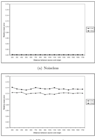
That is, the fan-beam model is approaching the parallel projections by increasingr. The effect of this change is shown in Fig. 6.
Both curves in Fig. 6 show that there is no big difference between the results when the source is close to or far from the origin. More gen-erally, there is no real difference between the fan-beam and parallel-beam projections if we change this distance. The Fig. 6(b)also shows
that we got better results when we used line in-tegrals to calculate the projections in the noisy case. In noisy experiments, the errors are higher in both cases.
0,00 0,02 0,04 0,06 0,08 0,10 0,12 0,14 0,16 0,18
250 350 450 550 650 750 850 950 1050 1150 1250 1350 1450 1550 1650 1750
Distance between source and origin
R
e
la
ti
ve
m
e
an
er
ro
r
Line Strip
(a) Noiseless
0,00 0,02 0,04 0,06 0,08 0,10 0,12 0,14 0,16 0,18
250 350 450 550 650 750 850 950 1050 1150 1250 1350 1450 1550 1650 1750
Distance between source and origin
R
e
la
ti
ve
m
ean
er
ro
r
Line Strip
(b) 5% Gaussian noise
Fig. 6. Relative mean error as a function of the distance between source and origin(r)for the line and strip
integrals whenK=32. There is no big difference
between the results when the source is close to or far from the origin.
4.2. Start Angle
We changed the value of the angle parameterθ0
between 0 and 360=Kdegrees. It is clear that by
determining the position of the first source we determine also the positions of all sources along the circleCr(if the number of sources is fixed).
Our previous results 9] show that there is no
significant difference in relative mean square if we have relatively large number of source points/projections.
However, we got different curves if the number of projections was small and there was some special direction in the image. For example, when the number of source points was K = 4,
0 0,1 0,2 0,3 0,4 0,5 0,6 0,7 0,8
0 5 10 15 20 25 30 35 40 45 50 55 60 65 70 75 80 85 90
Start angle
R
e
la
ti
ve
m
ean
er
ro
r
Line Strip
(a) Noiseless
0 0,1 0,2 0,3 0,4 0,5 0,6 0,7 0,8
0 5 10 15 20 25 30 35 40 45 50 55 60 65 70 75 80 85 90
Start angle
R
e
la
ti
ve
m
e
an
er
ro
r
Line Strip
(b) 5% Gaussian noise
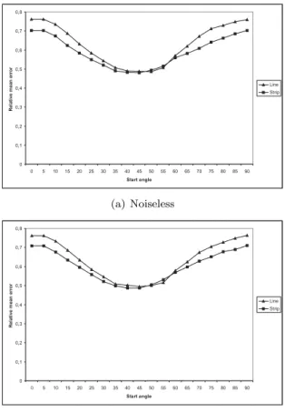
Fig. 7.Relative mean error as a function of the start angle(θ0)for the line and strip integrals whenK=4.
We got the best result when the start angle was around
θ0=40 .
It is noticeable that start angle aroundθ0=40
gave the best result in both cases of line and strip integrals. The reason is that in this case the image(Fig. 4(a))contains circles placed
al-most diagonally. In the curves corresponding to noisy projections this valley is also visible. We found that the relative mean errors were at the same level in noiseless and noisy cases as well. Considering the average time duration, we can say that in certain points the reconstruction algo-rithm using strip integrals takes approximately twice the time compared to the one using line integrals(Fig. 8).
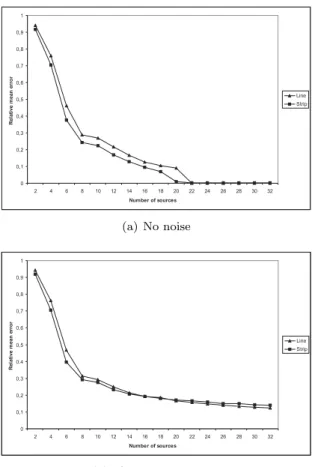
4.3. Number of Source Points
The number of source points (K), in other
words, the number of projections, was varied between 2 and 32 (Fig. 9). A natural
expec-tation is that the quality of the reconstruction
0 1 2 3 4 5 6 7 8 9 10
0 5 10 15 20 25 30 35 40 45 50 55 60 65 70 75 80 85 90
Start angle
T
im
e
(s
ec) Line
Strip
(a) Noiseless
0 1 2 3 4 5 6 7 8 9 10
0 5 10 15 20 25 30 35 40 45 50 55 60 65 70 75 80 85 90
Start angle
T
im
e
(sec) Line
Strip
(b) 5% Gaussian noise
Fig. 8.Time(sec)as a function of the start angle(θ0)
for the line and strip integrals whenK=4. Using strip
integrals takes approximately twice the time in certain points compared to using line integrals.
improves by increasing the number of projec-tions. The question here is, what is the (
rel-atively small) number from which the quality
changes very modestly.
The graphs in Fig. 9 show that the improve-ments is hardly recognizable beyond a certain value ofK.
In noiseless case, if we had sufficient number of equations for the unique determination of the linear equation(3), we reached the solution
at K = 20 when we used strip integrals and
K = 22 when we used line integrals. In the
noisy case line integrals gave better result from a certain number of sources.
In this experiment we can notice that the recon-struction always takes longer using strip inte-grals than using line inteinte-grals (Fig. 10). The
0 0,1 0,2 0,3 0,4 0,5 0,6 0,7 0,8 0,9 1
2 4 6 8 10 12 14 16 18 20 22 24 26 28 30 32
Number of sources
R
e
la
ti
v
e
m
e
a
n
e
rro
r
Line Strip
(a) No noise
0 0,1 0,2 0,3 0,4 0,5 0,6 0,7 0,8 0,9 1
2 4 6 8 10 12 14 16 18 20 22 24 26 28 30 32
Number of sources
R
e
la
ti
ve
m
e
an
er
ro
r
Line Strip
(b) 5% Gaussisan noise
Fig. 9.Relative mean error as a function of the number of sources(K)for the line and strip integrals. We
reached the solution atK=20 when we used strip
integrals andK=22 when we used line integrals. In the
noisy case, line integrals gave better result from a certain number of sources.
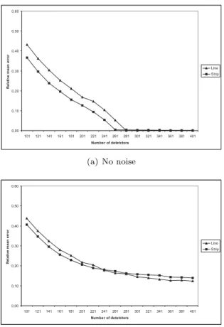
4.4. Number of Detector Elements
It is clear that if we have more detector ele-ments(L), we also have more equations in (3)
and, therefore, more information about the im-age. However, we cannot get better mean square error(Fig. ??(a))beyond a certain value of L,
hereL=261.
In the noisy case, the quality of the reconstruc-tion is improving almost everywhere in the pa-rameter interval(Fig. ??(b)). As a summary,
we can say that simply by increasing the num-ber of detector elements we reached substantial improvements only up to a certain limit(Ln).
5. Discussion and Conclusions
We have studied the geometric parameters of the fan-beam projections used in the
recon-0 10 20 30 40 50 60 70
2 4 6 8 10 12 14 16 18 20 22 24 26 28 30 32
Number of sources
T
im
e
(sec) Line
Strip
(a) No noise
0 10 20 30 40 50 60 70
2 4 6 8 10 12 14 16 18 20 22 24 26 28 30 32
Number of sources
T
im
e
(sec) Line
Strip
(b) 5% Gaussisan noise
Fig. 10.Time(sec)as a function of the number of
sources(K)for the line and strip integrals. The
reconstruction takes longer using strip integrals.
struction of binary matrices. Simulation exper-iments were performed by reconstructing phan-toms with different parameter settings.
We observed no remarkable difference between the line and strip integrals in the noiseless case when the distance between the source positions and the origin was large enough. The reason for the small differences between using strip and line integrals probably comes from the smooth-ing effect of the strip integral. If we have small number of sources, the start angle plays signif-icant role in the quality of the reconstruction in case of the given phantom.
In all other experiments, the differences caused by the two kinds of integrals in the computation of the projections were very small too. For the noiseless(ideal)case and for the noisy case, it
0,00 0,10 0,20 0,30 0,40 0,50 0,60
101 121 141 161 181 201 221 241 261 281 301 321 341 361 381 401
Number of detetctors
R
e
la
ti
ve
m
e
an
er
ro
r
Line Strip
(a) No noise
0,00 0,10 0,20 0,30 0,40 0,50 0,60
101 121 141 161 181 201 221 241 261 281 301 321 341 361 381 401
Number of detetctors
R
e
la
ti
ve
m
e
an
er
ro
r
Line Strip
(b) 5% Gaussian noise
Fig. 11.Relative mean error as a function of the number of detector elements(L)for the line and strip integrals
whenK=32. By increasing the number of detector
elements we reached substantial improvements only up to a certain limit(L n).
The final aim of these experiments was to get good parameter settings in a discrete tomogra-phy system to be realized in future applications. The results presented here can be used in plan-ning such physical imaging devices.
Acknowledgment
This work was supported by the OTKA grant T 048476 and NSF grant DMS0306215 (
As-pects of Discrete Tomography).
References
1] G.T. HERMAN, A. KUBA, Discrete
Tomogra-phy: Foundations, Algorithms, and Applications. Birkhauser, Boston,(1999).
2] R.A. BRUALDI, Matrices of zeros and ones with
fixed row and column sum vectors,Linear Algebra AppI. 33(1980)pp. 159–231.
3] A. KUBA, G.T. HERMAN,A historical introduction.
In1],(1999).
4] A.C. KAK, M. SLANEY,Principles of Computerized
Tomographic Imaging. New York, NY: IEEE Press, Inc.,(1988).
5] P. GRANGEAT, Mathematical framework of cone
beam 3D reconstruction via the first derivative of the Radon transform. Mathematical Methods in To-mography,Lecture notes in Mathematics, eds. G.T. Herman, A.K. Louis, and F. Natterer, 1497(1991),
pp. 66–97.
6] B. CHALMOND, F. COLDEFY, B. LAVAYSSIERE,
To-mographic reconstruction from non-calibrated noisy projections in non-destructive evaluation. Inverse Problems15(1999), pp. 399–411.
7] A. KUBA, L. RUSKO´, L. RODEK, Z. KISS,
Prelim-inary results of Discrete Tomography in Neutron Imaging. IEEE Trans. Nucl. Sci. 52 (2005), pp.
380–385.
8] N. ROBERT, F. PEYRIN, M.J. YAFFE, Binary vascular
reconstruction from limited number of cone beam projections.Med. Phys.21(1994), pp. 1839–1851.
9] A. NAGY, A. KUBA, Reconstruction of binary
ma-trices from fan-beam projections.Acta Cybernetica
17(2005), pp. 359–383.
10] N. METROPOLIS, A. ROSENBLUTH, M. ROSEN
-BLUTH, A. TELLER, ANDE. TELLER, Equation of
state calculation by fast computing machines.
J. Chem. Phys.21(1953), pp. 1087–1092.
11] A. KUBA, G.T. HERMAN, S. MATEJ, A. TODD
-POKROPEK, Medical applications of discrete
to-mography, inDIMACS Series in Discr. Math. and Theor. Comp. Sci.55(2000), pp. 195–208.
12] G.T. HERMAN, A. KUBA, Discrete tomography in
medical imaging, Proc. of IEEE 91 (2003), pp.
1612–1626.
Received:December, 2004 Revised:February, 2006; March, 2006 Accepted:April, 2006
Contact address: Antal Nagy Department of Image Processing and Computer Graphics University of Szeged ´Arp´ad t´er 2 H-6724 Szeged Hungary e-mail:[email protected]
ANTALNAGYis a research assistant at the Department of Image Process-ing and Computer Graphics, University of Szeged. His areas of interest include image processing, discrete tomography, and Picture Archiving and Communication Systems.
ATTILAKUBAis a Professor at the Department of Image Processing