A Feature Space-based Business Model Quality Evaluation Method

(1)

A Feature Space-based Business Model

Quality Evaluation Method

Zhongjie Wang, Xiaofei Xu and Dechen Zhan

School of Computer Science and Technology, Harbin Institute of Technology, China

It is inevitable that there are more or less diversities between business models created by different modelers, thus it is necessary to evaluate and compare them quanti-tatively to help decision makers discover whose models are pressing much closer to customer requirements. In this paper, a new approach for business model quality evaluation is presented. In order to deal with business models described by varied modeling languages, a uni-fied and extended feature modeling technique is adopted. Quality of a user-created model is then measured from two views, “completeness” and “soundness”, by assess-ing the distance between the user model and the standard model with the help of feature space as the tools. An example is briefly shown along with each concept and algorithm for illustration. Benefits and deficiencies of our method are briefly concluded for future works.

Keywords: business model, feature space, model quality evaluation, completeness, soundness

1. Introduction

“Business modeling” refers to the documenta-tion of a business system using a combinadocumenta-tion of text, graphical or formal notations, to clearly de-scribe reality and understand requirements ac-cordingly, to compute, reason, verify, design and develop software systems based on these business models. A consensus has been reached that business modeling plays an extremely im-portant role in the lifecycle of a software sys-tem (especially those complex enterprise soft-ware and applications, e.g., ERP, CRM, SCM)

to support computer integrated manufacturing management in modern enterprises.

Since “the achievement of software requirement quality is thefirst step towards software quality”

[1]and software requirements are primarily de-scribed by business models, if a business model

cannot exhibit those realistic requirements cor-rectly and completely, then it is destined that the final software systems are incorrect and incom-plete likewise.

However, business modeling has been consid-ered as a process which requires rich know-ledge and experiences about the business, i.e., if a modeler had no deep understandings on real-life business, the models he creates would be much more inferior than the models created by domain experts. Therefore, for a decision-maker in a CIM project, it is necessary to de-termine, when multiple modelers individually create their models for the same business re-quirements, whose models are better, i.e., to perform “business model quality evaluation”. In previous literatures, researches on model quality evaluation are mainly classified into the following four aspects:

• Evaluating the capacity of business mod-eling methodologies and languages, i.e., to judge whether a specific modeling ap-proach and its notations could satisfy those common or specific modeling require-ments. For example,[2] proposes a con-ceptual framework for comparing various reference models based on an elabora-tion of a linguistics-based classificaelabora-tion approach, _[3_] evaluates the capacity of UML and [4]evaluates UML interaction diagram, with detailed results to show the insufficiencies of UML and interaction di-agrams.

(2)

requirements documents to be used for de-tecting and removing defects that could cause errors in the transition to formal models. For UML-type models, a tool named DesignAdvisor was developed spe-cifically in[5]to analyze and measure the “goodness” of large, complex UML mod-els. _[6_] adopts the scenarios concept to evaluate the description of requirements. Aiming data models, [7] presents a set of quality factors(e.g., Simplicity, Com-pleteness, Correctness, Integrity, Flexibil-ity, etc) and the corresponding proposed metrics.

• Evaluating semantics soundness and per-formance of a model, e.g., for workflow models, identifying exceptional paths[8], verifying authorization reasonability [9], checking whether there are invalid paths

[10_] or whether the synchronization fea-ture might be preserved at runtime [11], etc. In these approaches, semantics per-formance is usually verified by simula-tion, and semantics soundness is usually verified by rule-based logical reasoning. • Evaluating runtime feasibility of a model,

e.g., estimating the cost and benefit of an e-business model from an economic value perspective [12], judging whether a sup-ply chain model has sufficiently quick re-sponse time and low operation cost_[13_], etc.

In above four aspects, the first one deviates from our subject ₍we focus on the quality of models instead of the modeling methodologies), the second one emphasizes syntax forms of the models, while the third and fourth ones focus on semantics quality.

Most of these approaches usually aim at some specific quality features of a specific model and the assessment results just reflect some defi-ciencies in the model. However, many quality factors could only be obtained after compari-son(with a standard model), e.g., completeness of a model; in addition, if there are no flaws on syntax, semantics and performance in two models, how to judge which one is better? Un-fortunately, most of the above approaches have neglected such situation.

Considering from another viewpoint, we may see that the above methods have provided differ-ent quality indicators of whose metrics is quite

related to the concrete forms of the models to be qualified, which makes their application scopes limited and there is a lack of a uniform evalua-tion method for any forms of models.

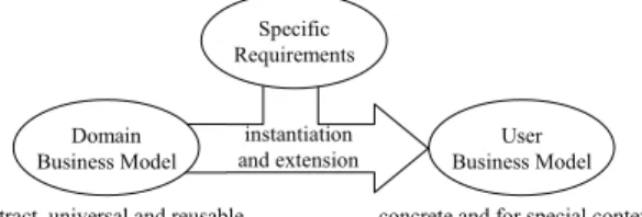
Firstly, we consider the issue “model compar-ison”. Currently, most popular modeling ap-proaches have already discarded the “from scratch” modeling way; on the contrary, after long-term accumulation domain experts have gathered and summarized those general know-ledge in each business domain and gathered rich domain models; when a concrete model is re-quired to be established, modelers may directly start from the domain model to carry on some re-visions according to specific requirements. This approach is shown in Figure 1.

User Business Model Specific

Requirements

abstract, universal and reusable concrete and for special context Domain

Business Model

instantiation and extension

Figure 1. Generating concrete business models from domain models and user requirements.

A model may be considered as a set ofmodel el-ementsandrelationshipsbetween them, the lat-ter of which may be considered and described as a set of rules or constraints on the former. Evaluating the quality of auser business model

(U₎ is comparing it with thedomain business model(D)andspecific requirements(R)to see whetherU contains necessary model elements in D and R(completeness)and whether the el-ements in U satisfy the constraints prescribed in D and R ₍soundness₎, in a word, it is quan-titative calculating the distance betweenU and D∩R. In the following discussions, we call D∩R astandard model(S).

(3)

The rest of this paper is arranged as follows. In Section 2, extended feature modeling method is briefly introduced. In Section 3, feature space-based model quality evaluation method is elab-orately proposed with a practical case. The con-clusion is given in Section 4.

2. Feature-oriented Business Model

As mentioned above, a business model is com-posed of a set of business elements and a set of relationships between these elements. Relation-ships between elements are classified into three types, i.e.,composition, generalizationand de-pendency, in whichcompositionorganizes busi-ness models as hierarchical structure, general-ization makes models reusable in different ap-plication scenarios and dependency describes semantics associations between the elements. The reason why we import and extend the feature-oriented modeling techniques[14][15][16]is that it has the ability to describe the three relation-ships in models.

2.1. Feature and Feature Space

Feature is an ontology that is used to describe the knowledge of external world, and is repre-sented as “Terms” or “Concepts” used to de-scribe the services supplied by a specific busi-ness domain, e.g., business processes,business activities,business objects,states attributesand

operations, etc.

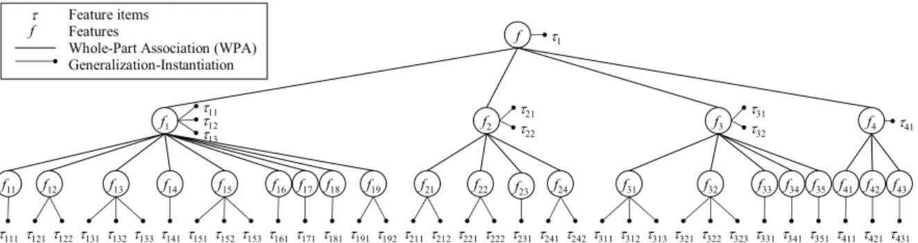
Features are hierarchical, i.e., there is a compo-sitionrelationship, or “whole-part association”, between parent and child features. According to this property, related features are organized as a multi-layer feature space, denoted asΩ=<F,

D >, in whichF is feature set andDis the set of feature dependencies between features inF. Ωis usually represented as the form offeature tree, where there is one and only one root fea-turefrootandchild(f),parent(f),ancestor(f), descendant(f)andsibling(f)are used to denote

f’s child feature set, parent feature set, ancestor feature set, descendant feature set and sibling feature set, respectively.

A feature item is an instance of a feature, de-scribes the feature’s one possible value under a given business environment, and reflects the

variability of the feature. Let dom(f) denote the set of all feature items of feature f, which is called the “domain” off. For∀τ ∈dom(f),

τ is called a value of f. A feature is an ab-straction of all its feature items, and there exists a generalization-instantiation association₍GIA₎ between a feature and its items.

The instantiation of a feature f is the pro-cess of choosing a proper feature item from

dom(f) for f to satisfy a specific semantics context, denoted as τ(f). Similarly, by instan-tiating a feature vectorY = (f1,f2, . . . ,fn), we

can get an instance of Y, denoted as τ(Y) = (τ(f1),τ(f2), . . .,τ(fn)), in which τ(fi) ∈

dom₍fi), 1 ≤ i ≤ n. If we instantiate each

feature f1,f2, . . . ,fn in Ω, we can get one of

Ω’s instance, denoted ast(Ω). All the instances ofΩconstituteΩ’s instance setT(Ω). It is easy to know thatT(Ω)⊆domf1)×dom(f2)×. . .× dom(fn), and∀t ∈ T(Ω), t = (τ1,τ2, . . . ,τn),

in whichτi ∈ dom(fi)is the projection oft on

fi, also denoted ast[fi]. t’s projection on feature

setX is denoted ast[X].

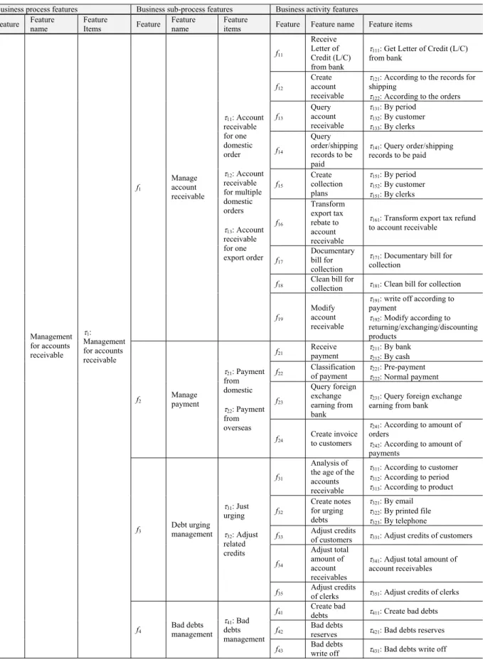
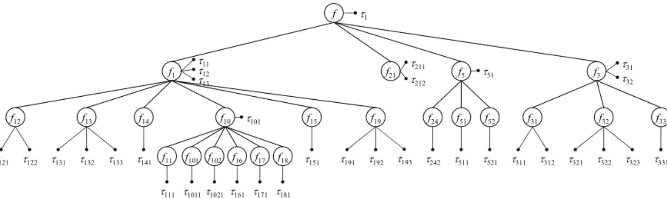
Figure 2 shows the feature space of a business model for “Account Receivable Management” in Enterprise Resource Planning₍ERP₎domain, Table 1 lists all the features and feature items in this model and Table 2 shows some of feature dependencies contained in the model. Due to limited space, here we only show those func-tional features₍e.g., business process and busi-ness activities₎and “execution order” relations between them.

2.2. Feature Dependency

In a feature spaceΩ=<F,D>,Dis the depen-dency set between features inF. As presented in our previous publications_[16_][17_], afeature dependency₍FD₎is defined as the relationships between two related features in a feature space. According to the structural and semantic rela-tionships between two features, FD can be clas-sified into five types:

• Whole-part Association(WPA)

• Feature Integrity Dependency₍FID₎ • Feature Value Dependency(FVD)

(4)

f

f1 f2 f3

f11 f12 f21 f22 f24 f31 f32 f33 f34

τ11

τ12

τ21

τ22

τ31

τ32

τ111 τ221 τ241τ242τ311τ312τ313τ321τ322τ323τ331τ341

f4

f13 f14 f15 f16 f17 f18 f19 f35 f41 f42 f43

τ421

τ411 τ431

τ1

τ41

τ121τ122τ131τ132τ133τ141 τ152 τ161τ171τ181τ191τ192τ211τ212 τ222 τ351

τ13 Feature items

f Features

τ

Whole-Part Association (WPA) Generalization-Instantiation

τ151 τ153

f23

τ231

Figure 2.Feature space for “Account Receivable Management” business model.

WPA is the simplest FD and represents fixed composition relationshipbetween child and par-ent features and explicitly behaves as the parpar-ent- parent-child structure.

FID is a dependency between a featuref and its child feature setY(i.e.,Y =child(f)), denoted asf_{| →}Y. It describes whether each feature in

Y would be selected as an essential part of f’s instance when f is instantiated. According to the number of features that are selected for f’s instantiation, there are four types of FIDs, i.e.,

mandatory FID,optional FID,single-selection FID and multiple-selection FID, denoted as

f_|M _→ _g_, _f_|O _→ _g_, _f_|S _→ _Y_, _f_|T _→ _Y

re-spectively.

• Mandatory FID (f|M _→ _g₎_{: no matter}

which instance f is instantiated, g is al-ways necessary;

• Optional FID(f|O _→ _g₎_: _g_{is necessary}

for some instances off, however, for other instances off, it is unnecessary;

• Single selection FID₍f_|S_→_Y₎_{: for each}

instance of f, there is one and only one feature for whichgis necessary;

• Multiple selection FID (f|T _→ _Y₎_{: for}

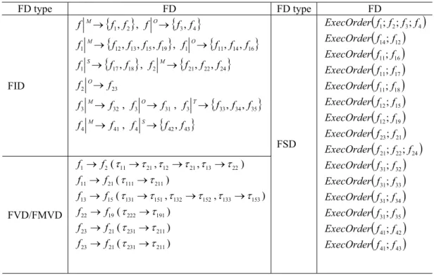
each instance off, there are possibly mul-tiple features for whichgis necessary; For example, in Figure 2, from the above defi-nitions we have(1)f1M → {f12,f13,f15,f19}

because f12, f13, f15, f19 are all necessary for

τ11,τ12 andτ13;(2)f1O→ {f11,f14,f16}

be-causef11,f14,f16are only necessary forτ13,τ12

andτ13 respectively;(3)f1S→ {f17,f18}

be-cause only one off17andf18may be required by

τ13at the same time;(4)f3T → {f33,f34,f35}.

FID can be regarded as the dependencies be-tween the “Values” of parent feature and the “Type” of its child features, therefore it is called

“Value-type” dependency, i.e., one feature item of parent feature determines which of child fea-tures are the essential parts of the parent feature. FID depicts the structural integrity relationships between parent and child features.

FVD and FMVD both depict the restrictions that must be satisfied when different features are instantiated, therefore they are called “ Value-value” dependency, i.e., the instances of one feature set uniquely or multiply determine the instances of another feature set. They generally appear between sibling features.

We use X → Y to denote the FVD betweenX

and Y and call “Y feature value dependent on X”. Similarly, X →→ Y is adopted to denote the FMVD betweenXandY.

For example, in Figure 2, when f1 is

instanti-ated as τ11 or τ12, f2 must have the valueτ21,

and whenf1is instantiated asτ13,f2must have

the valueτ22, therefore we havef1→f2.

Similar to functional dependency in relational model, FVD and FMVD also have the character-istics ofReflexivity,Augmentation,Transitivity,

Pseudotransitivity, Union and Decomposition, etc. According to Armstrong Axiom _[18_], we can get a feature set X’s closure on FD set D, denoted asX+, which contains all the features that directly or indirectly depend on features in

X.

FSD refers to the semantics association between features. It is irrespective with the values of fea-tures, and it represents constraints between the

typeof related features, i.e., a “Type-type” de-pendency. FSD is essentially a set of constraints with the following possible types:

(5)

Business process features Business sub-process features Business activity features

Feature Feature_name Feature_Items Feature Feature_name Feature_items Feature Feature name Feature items

f11

Receive Letter of Credit (L/C) from bank

W111: Get Letter of Credit (L/C) from bank

f12

Create account receivable

W121: According to the records for shipping

W122: According to the orders

f13

Query account receivable

W131: By period

W132: By customer

W133: By clerks

f14

Query order/shipping records to be paid

W141: Query order/shipping records to be paid

f15

Create collection plans

W151: By period

W152: By customer

W151: By clerks

f16

Transform export tax rebate to account receivable

W161: Transform export tax refund to account receivable

f17

Documentary bill for collection

W171: Documentary bill for collection

f18 Clean bill for _collection W181: Clean bill for collection f1

Manage account receivable

W11: Account receivable for one domestic order

W12: Account receivable for multiple domestic orders

W13: Account receivable for one export order

f19

Modify account receivable

W191: write off according to payment

W192: Modify according to returning/exchanging/discounting products

f21 Receive_payment W211: By bank

W212: By cash

f22 Classification_{of payment} W221: Pre-payment

W222: Normal payment

f23

Query foreign exchange earning from bank

W231: Query foreign exchange earning from bank f2 Manage _payment

W21: Payment from domestic

W22: Payment from overseas

f24 Create invoice _{to customers}

W241: According to amount of orders

W242: According to amount of payments

f31

Analysis of the age of the accounts receivable

W311: According to customer

W312: According to period

W313: According to product

f32

Create notes for urging debts

W321: By email

W322: By printed file

W323: By telephone

f33 Adjust credits _{of customers} W331: Adjust credits of customers

f34

Adjust total amount of account receivables

W341: Adjust total amount of account receivables f3 Debt urging _management

W31: Just urging

W32: Adjust related credits

f35 Adjust credits _{of clerks} W351: Adjust credits of clerks

f41 Create bad _debts W411: Create bad debts

f42 Bad debts _reserves W421: Bad debts reserves f Management for accounts

receivable

W1:

Management for accounts receivable

f4 Bad debts _management

W41: Bad debts management

f43 Bad debts _{write off} W431: Bad debts write off

(6)

D F e

O_→

{

17 18

}

1 f ,f f S_→

, f2

{

f21,f22,f24

}

M_→

23

2 f

f O_→

32

3 f

f M_→

, f3 f31

O_→

, f3

{

f33,f34,f35

}

T_→

41

4 f

f M_→

, f4

{

f42,f43

}

S_→

FVD/FMVD

2 1 f

f → (τ11→τ21,τ12→τ21,τ13→τ22)

21 11 f

f → (τ111→τ211)

15 13 f

f → (τ131→τ151,τ132→τ152,τ133 →τ153)

19 22 f

f → (τ222→τ191)

21 23 f

f → (τ231→τ211)

ExecOrder

Table 2.Feature dependencies in the example model.

condition C is true, can a role R have the right to execute activity A;

• Numerical association rule [20] in busi-ness object model describes the associa-tion between different business objects, e.g., the “Generated from” association between Purchasing Requirement object andPurchasing Orderobject, or the “ Al-located to” association betweenSale Or-derobject andCustomer Paymentobject. • ECA rule[21]in business process model describes the execution order between dif-ferent business activities, i.e., only when events E occurs and condition C is true, can activity A be allowed to execute; after A’s execution, it generates new events E’. For example, in Figure 2, the execution order of

f1,f2,f3,f4must bef1 →f2→f3 →f4,

there-fore we have a FSDExecOrder(f1;f2;f3;f4).

2.3. Feature Space Partition

A business model is reusable, but when it is ap-plied for a specific requirement, its feature space should be instantiated as a semi-abstract or fully concrete model₍i.e., those features and feature items that are used for other requirements are

not necessarily contained). Therefore, the fea-ture space of a business model may be parti-tioned into two parts: mandatoryandoptional

parts. The partition basis is the constraints ex-pressed by feature dependencies.

3. Model Quality Evaluation Based on Feature Space Matching

In this section, with the aid of feature space as the uniform form of based business models, we design a model quality evaluation method. The basic evaluation process is to semi-automatically compare and analyze the feature spaces between user model and standard model to measure the distance(“gap”)between them. Larger distance indicates that the user model is far more incon-sistent with the standard model, therefore it has lower quality.

Such distance will be assessed from two points of view: completeness and soundness. Com-pleteness indicates where user model contains necessary elements of standard model, while

soundness indicates whether user model holds those necessary constraints in standard model. In the following discussion, we will useΩS ₌

(7)

ΩU ₌ _FU_,_DU _{as the} _{user model} ₍_U₎_{. To}

illuminate our method with an example, we will use the model in Figure 2 as Sand use Figure 3 as U to evaluate the quality of U compared with S. Table 3 shows the meanings of those new features that appear inU.

Features or

Feature Items Meanings

f10 Accounts receivable for export f1011 Export tax refund filing f1021 Transfer Letter of Credit(L/C)

f5 Invoice management

f51 Audit invoice

f52 Cancel invoice

τ101 Accounts receivable for export

τ193 Write off account receivable_{according to pre-payment}

τ51 Invoice management

Table 3. New features and feature items in user model.

3.1. Completeness

Generally speaking, completeness indicates whether a user model contains the mandatory parts of the standard model. No containing or partial containing means it is possible that some functions are lost inU, orU’s application scope is narrowed. The more lost functions there are, the less completenessU has.

Aiming at feature space-based business models,

completenessis measured from two aspects:

(1) Which mandatory features (in S) are not contained in U? If a mandatory feature f inS

does not exist in U, functions of f will not be supported inU;

(2) Which mandatory feature items (in S) are not contained in U?If a mandatory feature item

τoff inSdoes not exist inU, thenUcannot be reused in the specific domain provisioned byτ

off, thereforeU’s application scope is reduced.

Definition 1. (Completeness Matching Degree

ω) The completeness matching degree of U

compared with S is defined as the proportion of the number of mandatory features(inS) con-tained inU, compared with the total number of mandatory features(inS).

We use algorithms 1 and 2 to calculateω. Algorithm 1₍Generating the mandatory feature set of a feature)

GenerateMandatoryPart(f,T,S)

Input: Ω=_FS_,_DS_, _f _∈ _FS_, _T _⊆ _domS₍_f₎_{, where} domS₍_f₎_{denotes the domain of}_f _{when it is in}_S_; Output:MP

Step 1: Set the domain off asT, addf intoMPand set f and all its feature items with flag 1;

Step 2: Select one featuregwith no flag fromMPand supposedomS₍_g_{) =}_Q_;

Step 2.1: Select one feature itemτwith no flag from Qwith the essential sub-feature set es set(τ); Step 2.1.1: If es set(τ) =∅, then go to Step 2.1.4; Step 2.1.2:∀k∈es set(τ), find those FVD/FMVDs

(fromDS₎_between_f _and_k_{; then} accord-ing to these FVD/FMVDs, choose those mandatory feature items of k, denoted asτ(k) (i.e., whenf is instantiated asτ, kshould be instantiated as any items in τ(k));

Step 2.1.3: Ifk∈MP, letdom(k) =dom(k)∪τ(k); otherwise, letdom(k) =τ(k)and addk toMP;

Step 2.1.4: Setτwith flag 1 and continue to execute Step 2.1 until there are no suchτ;

f

f1 f3

f11

f12

f21 f5

f31 f32 f33

τ11

τ12 τ_τ31

32

τ111

τ323 τ331

τ322

τ311 τ312 τ321

f13 f14 f15

f16 f17 f18

f19

τ1

121 τ122 τ131 τ132 τ133 τ141 τ151

τ161 τ171 τ181

τ191 τ192

τ211

τ212

τ13

f24 f51 f52

τ511 τ521

f10

f101 f102

τ1011τ1021

τ242

τ193

τ101

τ51

τ

(8)

Step 2.2: If there are no suchgin Step 2, the algorithm ends. NowMPcontains f’s all mandatory descendant features and the corresponding feature items.

Algorithm 2(Calculating the completeness mat-ching degree betweenUandS)

CalculateMatchDeg(U,S)

Input:Ω=_FS_,_DS_, _ΩU₌_FU_,_DU Output: ω

Step 1: Suppose the root feature ofSisf, with the doma-inT =domS₍_f₎_{. Call Algorithm 1 to generate} f’s mandatory descendant features and feature items inS, i.e.,MP=GenerateMandatoryPart

(f,T,S);

Step 2: Calculate the number of features/feature items contained inMP, i.e.,N=|MP|,

M=

g∈MP|dom(g)|;

Step 3: Letn=0,m=0, and∀g∈MP, Step 3.1: Ifg∈/FU_{, let}_n₌_n₊_1;

Step 3.2: Ifg∈FU_{, then}_∀_τ_∈_domU₍_g₎_{, if}_τ_∈_/ domS₍_g₎_{, let} _m₌_m₊_{1. Repeat Step 3.2} until all the feature items of g have been checked;

Step 3.3: Repeat Step 3 until allghas been checked;

Step 4: ω=1−_Nn×1−_Mm.

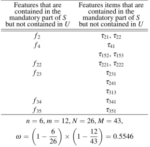
Here we use the algorithm for the example, and the results are shown in Table 4.ω =0_.5546 in-dicates that only 55_.46% mandatory elements in standard model are contained in the user model to be evaluated.

Features that are contained in the mandatory part ofS but not contained inU

Features items that are contained in the mandatory part ofS but not contained inU

f2 τ21,τ22

f4 τ41

τ152,τ153

f22 τ221,τ222

f23 τ231

τ241

τ313

f34 τ341

f35 τ351

n=6,m=12,N=26,M=43,

ω=

1−₂₆6 ×

1−12₄₃ =0.5546

Table 4.Calculating the completeness matching degree betweenUandSin the example.

3.2. Soundness

Generally speaking,soundnessindicates whether

Upreserves the semantics constraints inS. The more destroyed constraints there are in U, the less soundnessU has.

Aiming at feature space-based business models

(in which semantics constraints are expressed as FDs), soundness may be mainly measured from the following four aspects:

(1)Soundness of composition relationships be-tween features (WPA). If some WPA are de-stroyed, then even ifUcontains all the manda-tory features in S, it will still lead to chaos of feature organizations, which will deteriorate the maintainability and understandability of mod-els;

(2)Soundness of instantiation relationships be-tween features₍FVD_/FMVD₎. If some of FVD_/ FMVD are destroyed, then the reuse scope of related features will be widened and lead to un-allowed interpretations of the models;

(3₎ Soundness of integration relationships be-tween features ₍FID₎. If some of FID are de-stroyed, then the reuse scope of related features will also be widened;

(4₎ Soundness of semantics dependency be-tween features₍FSD₎. If some of FSD are de-stroyed, model semantics will be lost or inten-sified.

Definition 2. ₍Soundness Matching Degreeθ)

Thesoundness matching degreeofUcompared withS is defined as the degree that ₍1₎U pre-serves the semantics constraints in S and (2)

the semantics constraints inU destroy the con-straints inS.

In the following subsections, we will present the metrics of θ aiming at four types of FD respectively.

3.2.1. WPA Soundness

(9)

andS to assess the WPA soundness by consid-ering five types of matching between U andS, i.e., the degree that WPA inUsatisfies the WPA inS.

The five types of matching are imported from

[22_].

• Embedded Matching (EM). This is the soundest matching, in which all the WPA have been preserved and the number of children of a feature is equal inUand in

S.

• Area Matching(AM). Similar to EM, all the WPA are also preserved, whereas the number of children of a feature in U is larger than the number of children of the same feature inS.

• Containment Matching₍CM₎. The WPA inSpossibly no longer maintains inU, but all the Ancestor-Descendant relationships inSare certain to maintain inU.

• Strong Constrained Containment Match-ing₍SCCM₎. Based on CM, SCCM should also follow the rule that if there are no Ancestor-Descendant relationships be-tweenf1,f2,f3, then

|ancestor₍f1)∩ancestor(f2)|

=|ancestor(f1)∩ancestor(f3)| ∈DS

⇔

|ancestor(f1)∩ancestor(f2)|

=|ancestor₍f1)∩ancestor(f3)| ∈DU

• Weak Constrained Containment Match-ing (WCCM). Based on CM, WCCM should also follow the rule that if there are no Ancestor-Descendant relationships betweenf1,f2,f3, then

|ancestor₍f1)∩ancestor(f2)|

<|ancestor(f1)∩ancestor(f3)| ∈DS

⇔

|ancestor(f1)∩ancestor(f2)|

≤ |ancestor(f1)∩ancestor(f3)| ∈DU

It is easy to see that the matching degree of the five types is: EM→AM→SCCM→WCCM→ CM, where an arrow aims at a more loose match-ing from a more tight one. For more discussions about these matchings, please refer to[22].

IfU andS satisfy one of the above matchings, the WPA soundness matching degree between them may be measured by calculating the num-ber of editing operations (e.g., insert, delete

ormodify features_/feature items_/WPA₎which makeU accord withS. The larger the number is, the smaller WPA soundness should be, and vice versa.

Algorithm 3(WPA soundness matching degree)

CalculateWPAMatchDegree(U,S)

Input:U,S Output:θWPA

Step 1: Judge which types of matching are possible betweenUandS;

Step 2: Calculate the editing cost for each matching betweenUandSand find the matching with the smallest editing costγ;

Step 3: Calculate thetotal sizeofS, i.e., K=FS₊

f∈FS

|dom(f)|+

f∈FS

|child(f)|;

Step 4:θWPA=exp−_Kγ.

In step 1, we may directly import the Gener-icMatchingalgorithm from [22] and use some specific optimization strategies(e.g., [23][24])

to reduce the time complexity. Due to limited space, we will not introduce the concrete pro-cess of these algorithms.

Using Figure 3 as an example, the WPA sound-ness matching degree between

• S and U1 is exp−0₅ = 1 (U does not

need any revision);

• S andU2 is exp−₅1 = 0.819(gshould

be deleted);

• S andU3 is exp−₅4 = 0.449(deleteg

andh, setf4andf5as the children off2);

• S andU4is exp−₅6 =0.301(insertf2

as a child off1, delete the WPA between f4,f5 andf1, setf4andf5as the children

off2);

• S and U5 is exp−7₅ = 0.247 (delete g, insert f2 as a child off1, set f4 as the

children off2, delete the WPA betweenf5

andf1, setf5 as the children off2, setf3

as the children off1);

(10)

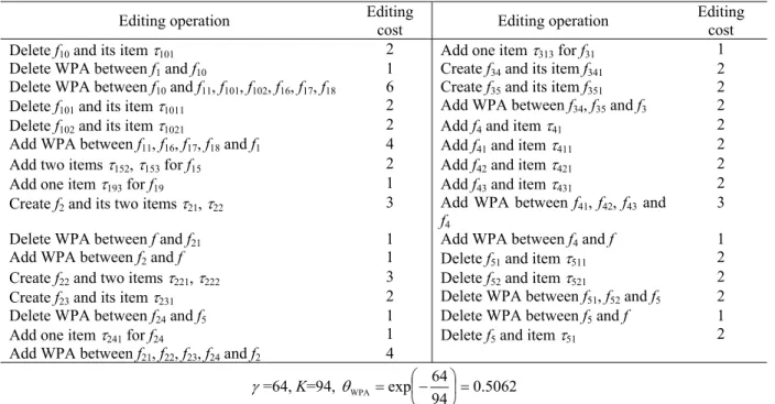
Editing operation Editing _cost Editing operation Editing _cost

Deletef10 and its item W101 2 Add one item W313 for f31 1

Delete WPA between f1 and f10 1 Create f34 and its item f341 2

Delete WPA between f10 and f11,f101,f102,f16,f17,f18 6 Create f35 and its item f351 2

Deletef101 and its item W1011 2 Add WPA between f34,f35 and f3 2

Deletef102 and its item W1021 2 Add f4 and item W41 2

Add WPA between f11,f16,f17,f18 and f1 4 Add f41 and item W411 2

Add two items W152,W153 for f15 2 Add f42 and item W421 2

Add one item W193 for f19 1 Add f43 and item W431 2

Createf2 and its two items W21,W22 3 Add WPA between f41,f42,f43 and f4

3

Delete WPA between f and f21 1 Add WPA between f4 and f 1

Add WPA between f2 and f 1 Deletef51 and item W511 2

Createf22 and two items W221,W222 3 Deletef52 and item W521 2

Createf23 and its item W231 2 Delete WPA between f51,f52 and f5 2

Delete WPA between f24 and f5 1 Delete WPA between f5 and f 1

Add one item W241 for f24 1 Deletef5 and item W51 2

Add WPA between f21,f22,f23,f24 and f2 4

J=64,K=94, 0.5062 94

64 exp

WPA ¸

¹ · ¨ © § T

Table 5.Editing operation list and the WPA soundness matching degree for the example.

3.2.2. FVD_/FMVD Soundness

An FVD/FMVD describes the dependencies between values of two sets of features. If an FVD_/FMVD exists inS, but does not inU, this means that the instantiation of related features in

Uis no longer constrained by this FVD/FMVD, which enlarges the reuse scope ofU. Otherwise, if an FVD/FMVD exists inU, but does not inS, it will reduce U’s reuse scope. Both situations are inadvisable.

Algorithm 4 ₍FVD_/FMVD soundness match-ing degree)

Input:S,U;

Output: θFVD;

Step 1: Suppose Θ =FS_∩_FD_{, then try to obtain the}

Θ’s feature closure inSandUrespectively, ac-cording to Armstrong axiom, denoted as ΘS∗

andΘU∗_{, and let}_Σ₌_ΘS∗_∩_ΘU∗_;

Step 2: According to the instantiation process, get Σ’s all possible instances in S and U respectively, denoted asTΣS_and_T_ΣU_;

Step 3:θFVD=1−

_T

ΣU₋_T_ΣS |T(ΣS₎_|

.θFVD<1

indi-cates that there ∃t ∈ TΣU _but _t _∈_/ _T_ΣS_, therefore the reuse scope ofUis larger thanS.

In the example, we have Θ =FS∩FD

={f, f1, f3, f11, f12, f13, f14, f15, f16, f17, f18, f19, f21, f24, f31, f32, f33},

TΣS₌_648,_T_ΣU₋_T_ΣS₌_136,

therefore

θFVD =1−

TΣU₋_T_ΣS

|T₍ΣS₎_|

=1−

136 648

=0.7901.

3.2.3. FID Soundness

Algorithm 5₍FID soundness matching degree₎ Input:U,S

Output:θFID

Step 1: LetΘ=FS_∩_FD_;

Step 2:∀f ∈Θ, according to the FIDs betweenf and its child features, calculate the following four sets off both inUandS, respectively,

• Mandatory feature set

MandatoryS₍_f₎_,_MandatoryU₍_f₎_; • Optional feature set

OptionalS₍_f₎_,_OptionalU₍_f₎_; • Single selection feature set

(11)

• Multiple selection feature set

MultipleSelectionS₍_f₎_,_{MultipleSelection}U₍_f₎_. Step 3: ∀f ∈Θ, calculate the FID soundness matching

degree betweenUandS, i.e.,

FIDMatchDeg(f) =

1 4 ×

MS(_|fMS)−(MUf)|(f)

+OS(_|f_OS)−₍OU_f₎_|(f) +SS(_|f_SS)−₍SU_f₎_|(f)+TS(_|f_TS)−₍_fTU₎_|(f)

Step 4: θFID= _|_Θ1_|

f∈ΘFIDMatchDeg(f). In the example, we have

θFID= _|Θ|1

f∈Θ

FIDMatchDeg₍f_{) =}0_.7920

(Detailed measurement process is ignored here₎.

3.2.4. FSD Soundness

Because different types of FSD are quite varied, it is difficult to provide a uniform strategy for FSD soundness evaluation, but the basic process may be summarized as follows:

(1) Check whether the model elements in U

fully satisfy each constraint of FSD inSor not;

(2₎ Check whether the FSD in U destroys the constraints of FSD inSor not.

In practice, specific evaluation methods must be carefully invented for each type of FSDs

(e.g., ECA rules, numeric association rules, ECA rules, etc). Due to limited space we will not show the details of these methods.

For our example, we haveθFSD=0.8735.

3.2.5. Integrated Soundness

Four types of soundness are integrated together to get the final soundness between U and S. However, the four types of soundness should not be considered as having the same impor-tance. According to our experience, we con-sider that the order of their weightiness may be

θWPA >θFSD >θFVD>θFIDand their weights

are specified as 0.45, 0.3, 0.15 and 0.1. There-fore, the integrated soundness is calculated by

θ =0.45×θWPA+0.3×θFSD

+0.15×θFVD+0.1×θFID

So in the example, we have

θ =0_.45_×0_.5062₊0_.3_×0_.8735

+0.15×0.7901+0.1×0.7920

=0.6876.

3.3. Total Evaluation

In subsections 3.1 and 3.2 we have introduced two metrics for business model quality evalua-tion, i.e.,completenessandsoundness, and the final quality ofUcompared withSmay be cal-culated byMatchDeg(U,S) =0.5×(ω +θ). In our practice, the following standards are adopted by decision-makers to determine whe-ther a user model is acceptable or not:

• MatchDeg₍U_,S_≥0_.8: Uis “good”; • 0.5≤ MatchDeg(U,S)< 0.8: U is “

ac-ceptable”;

• 0.3 ≤ MatchDeg(U,S) < 0.5: U is “bad”;

• MatchDeg(U,S) < 0.3: U is “ unaccept-able”.

In the example, we have

MatchDeg₍U_,S_{) =}0_.5_×₍ω +θ)

=0.5×(0.5546+0.6876)

=0_.6211_.

It means that the consistency between the user model U in Figure 3 and the standard model

S in Figure 2 is 62.11% and we may draw the conclusion thatUis an “acceptable” model and needs slight revisions.

4. Practical Validation

We applied the evaluation method in a course named “Enterprise Resource Planning: Design and Practice” in the semester of spring 2006. Aiming at a specific business domain “ Pur-chase Requirement and Order Management”, we asked each student to build their user model

(using feature space as modeling language)

(12)

we applied our evaluation method on them and got the following results:

MatchDeg Number of student models

[0.8, 1] 5(17.9%) [0.5, 0.8) 11(39.3%) [0.3, 0.5) 9(32.1%)

(0, 0.3) 3(10.7%)

Table 6.Results of experiments during the course. Then, two assistant instructors who both had wide experience inpurchasedomain, manually evaluated these models and got similar results. This showed that our method was consistent with reality and applicable in practice.

5. Conclusions

In order to solve the problem of “how to quan-titatively evaluate and compare the quality of business models”, we propose a new approach for business model quality evaluation, based on feature space with the following contributions:

• Based on the traditional feature modeling techniques, we extend them and import the concept “feature dependency” to uni-formly express various forms of business models.

• We measure the distance between user model and standard model from two view-points, i.e., completeness and soundness. • Completeness is used to judge whether a user model contains necessary model el-ements in the standard model. It can be measured by examining the integrity of features and feature items.

• Soundness is used to judge whether vari-ous constraints in a user model can satisfy and not destroy all the constraints inS. It can be measured by examining FD’s di-versity betweenUandS.

However, our method still has some shortcom-ings, e.g.,

• Although feature modeling is useful, it is complex to transform other forms of models into feature space-based models. In addition, such form of models seems

to lack the ability to describe process-oriented business model;

• We have not yet found a uniform form for various types of FSD, therefore we do not have such a uniform algorithm to evaluate FSD soundness.

• Since business models and information system are both socio-technical systems and not purely technical ones, formal and fully automatic evaluation might be cum-bersome, problematic, and leads to irrel-evant results.

Further research should address such issues.

References

[1] F. FABBRINI, M. FUSANI, S. GNESI, G. LAMI, An

Au-tomatic Quality Evaluation for Natural Language Requirements.Proceedings of the Seventh Interna-tional Workshop on RE: Foundation for Software Quality,(2001)Interlaken, Switzerland.

[2] B. VOJISLAV, J. MISIC, L. ZHAO, Evaluating the

Quality of Reference Models. Proceedings of the 19th International Conference on Conceptual Mod-eling, LNCS 1920/2000,(2000), 484–498, Salt Lake City, Utah, USA.

[3] J. KROGSTIE, Evaluating UML Using a Generic

Quality Framework. In UML and the Unified Pro-cess, L. Favre, Ed.,(2003), 1–22, IDEA Group.

[4] C. GLEZER, M. LAST, E. NACHMANY, P. SHOVAL,

Quality and Comprehension of UML Interaction Diagrams: an Experimental Comparison. Informa-tion and Software Technology,10(2005), 675–692.

[5] B. BERENBACH, Evaluating the Quality of a UML

Business Model. Proceedings of the 11th IEEE International Conference on Requirements Engi-neering,(2003)Stanford, CA, USA.

[6] M. GLINZ, Improving the Quality of Requirements

with Scenarios.Proceedings of the Second World Congress for Software Quality, (2000), 55–60, Yokohama, Japan.

[7] D. L. MOODY, Measuring the Quality of Data

Mod-els: an Empirical Evaluation of the Use of Quality Metrics in Practice.Proceedings of the 11th Euro-pean Conference on Information Systems, (2003)

Naples, Italy.

[8] H. B. LI, D. C. ZHAN, X. F. XU,Semantic Relation

Based Exception Detection in Workflow Systems. International Journal of Computer Science and Network Security, 2B(2006), 160–165.

[9] V. ATLURI, W. K. HUANG, A Petri Net-based Safety

(13)

[10] H. B. LI, D. C. ZHAN, Invalid Path Identification

of Workflow.Computer Integrated Manufacturing System,5(2006), 692-696.

[11] J. Z. CAI, S. K. ZHANG, L. F. WANG, Correctness

Verification of Synchronization-based Workflow Model. Proceedings of 2005 IEEE International Conference on e-Business Engineering, (2005), 527–530, Beijing, China.

[12] J. GORDIJN, H. AKKERMANS, Designing and Evalu-ating e-Business Models.IEEE Intelligent Systems,

4(2001), 11–17.

[13] L. LIU, S. JAIN, S. J. TURNER,ET AL., Distributed

Supply Chain Simulation across Enterprise Bound-aries.Proceedings of the Winter Simulation Confer-ence,(2000), 1245–1251, San Diego, CA, USA.

[14] K. C. KANG, S. G. COHEN, J. A. HESS, ET AL.,

Feature-oriented Domain Analysis (FODA) feasi-bility study. Technical Report, CMU/ SEI-90-TR-21, Pittsburgh: Carnegie Mellon University, Soft-ware Engineering Institute,(1990).

[15] K. C. KANG, S. KIM, J. LEE, ET AL., FORM:

A Feature-oriented Reuse Method with Domain-specific Reference Architectures. Annals of Soft-ware Engineering,5(1998), 143–168.

[16] Z. J. WANG, X. F. XU, D. C. ZHAN, A Component

Optimization Design Method Based on Variation Point Decomposition.Proceedings of the 3rd ACIS International Conference on Software Engineering, Research, Management and Applications,(2005), 399–406, Mt. Pleasant, Michigan, USA

[17] Z. J. WANG, X. F. XU, D. C. ZHAN, Feature-based

Component Model and Normalized Design Process. Journal of Software,1(2006), 39–47.

[18] W. W. ARMSTRONG, Dependency Structures of Data Base Relationships. Proceedings of Interna-tional Federation for Information Processing (IFIP) Congress 74,(1974), 580–583, Stockholm, North-Holland.

[19] R. SANDHU, E. COYNE, H. FEINSTEIN, H., ET AL.,

Role-based Access Control Models. IEEE Com-puter,2(1996), 38–47.

[20] Z. J. WANG, X. F. XU, D. C. ZHAN, A Log-based and Traceability-oriented Business Object Association Model for Code Generation.International Journal of Computer Science and Network Security, 3A 2006), 122–129.

[21] F. BRY, M. ECKERT, P. L. PATR˘ ANJANˆ , I. ROMA

-NENKO, Realizing Business Processes with ECA Rules: Benefits, Challenges, Limits. Proceedings of the 4th Workshop on Principles and Practice of Semantic Web Reasoning,(2006)Budva, Montene-gro.

[22] Y. F. WANG, Y. J. XUE, Y. ZHANG,ET AL., A

Match-ing Model for Software Component Classified in Faceted Scheme. Journal of Software, 3 (2003), 401–408.

[23] P. KILPELAINEN, Trees Matching Problems with

Applications to Structured Text Database. Ph. D. Thesis, Department of Computer Science, Univer-sity of Helsinki,(1992).

[24] D. SHASHA, J. TSONG, L. WANG, Exact and

Ap-proximate Algorithm for Unordered Tree Matching. IEEE Transactions on Systems Man and Cybernet-ics,4(1994), 668–678.

Received:October, 2006

Revised:June, 2007

Accepted:June, 2007

Contact addresses:

Zhongjie Wang Harbin Institute of Technology School of Computer Science and Technology West Dazhi Street 92, Harbin, China e-mail:[email protected]

Xiaofei Xu Harbin Institute of Technology School of Computer Science and Technology West Dazhi Street 92, Harbin, China e-mail:[email protected]

Dechen Zhan Harbin Institute of Technology School of Computer Science and Technology West Dazhi Street 92, Harbin, China e-mail:[email protected]

ZHONGJIEWANGis an associate professor at the Harbin Institute of Technology, Harbin, China. His research fields include enterprise and software modeling, software engineering, service-oriented computing and service engineering. He teaches Software Architecture, Introduc-tion to Service Sciences, and Software Engineering.

XIAOFEIXUreceived his PhD degree in Computer Science from Harbin

Institute of Technology in 1988. He is currently a professor, head of School of Computer Science and Technology and School of Software at the Harbin Institute of Technology, Harbin, China. He has more than 300 research papers presented in journals and at conferences. His research interests include database, computer integrated manufacturing (CIM), service sciences, decision support system(DSS), etc.