* Université Libre de Bruxelles, Service of Analysis of the Data (SAD), Bruxelles, BE
† Eindhoven University of Technology, Human Technology Interaction Group, Eindhoven, NL
Corresponding author: Marie Delacre ([email protected]) RESEARCH ARTICLE
Why Psychologists Should by Default Use Welch’s
t-test
Instead of Student’s t-test
Marie Delacre
*, Daniël Lakens
†and Christophe Leys
*When comparing two independent groups, psychology researchers commonly use Student’s t-tests. Assumptions of normality and homogeneity of variance underlie this test. More often than not, when these conditions are not met, Student’s t-test can be severely biased and lead to invalid statistical inferences. Moreover, we argue that the assumption of equal variances will seldom hold in psychological research, and choosing between Student’s t-test and Welch’s t-test based on the outcomes of a test of the equality of variances often fails to provide an appropriate answer. We show that the Welch’s t-test provides a better control of Type 1 error rates when the assumption of homogeneity of variance is not met, and it loses little robustness compared to Student’s t-test when the assumptions are met. We argue that Welch’s t-test should be used as a default strategy.
Keywords: Welch’s t-test; Student’s t-test; homogeneity of variance; Levene’s test; Homoscedasticity;
statistical power; type 1 error; type 2 error
Independent sample t-tests are commonly used in the psychological literature to statistically test differences between means. There are different types of t-tests, such as Student’s t-test, Welch’s t-test, Yuen’s t-test, and a boot-strapped t-test. These variations differ in the underlying assumptions about whether data is normally distributed and whether variances in both groups are equal (see, e.g., Rasch, Kubinger, & Moder, 2011; Yuen, 1974). Student’s
t-test is the default method to compare two groups in
psy-chology. The alternatives that are available are consider-ably less often reported. This is surprising, since Welch’s
t-test is often the preferred choice and is available in
prac-tically all statistical software packages.
In this article, we will review the differences between Welch’s t-test, Student’s t-test, and Yuen’s t-test, and we suggest that Welch’s t-test is a better default for the social sciences than Student’s and Yuen’s t-tests. We do not include the bootstrapped t-test because it is known to fail in specific situations, such as when there are unequal sam-ple sizes and standard deviations differ moderately (Hayes & Cai, 2007).
When performing a t-test, several software packages (i.e., R and Minitab) present Welch’s t-test by default. Users can request Student’s t-test, but only after explic-itly stating that the assumption of equal variances is
met. Student’s t-test is a parametric test, which means it relies on assumptions about the data that are ana-lyzed. Parametric tests are believed to be more powerful than non-parametric tests (i.e., tests that do not require assumptions about the population parameters; Sheskin, 2003). However, Student’s t-test is generally only more powerful when the data are normally distributed (the assumption of normality) and the variances are equal in both groups (homoscedasticity; the assumption of homo-geneity of variance; Carroll & Schneider, 1985; Erceg-Hurn & Mirosevich, 2008).
When sample sizes are equal between groups, Student’s
t-test is robust to violations of the assumption of equal
variances as long as sample sizes are big enough to allow correct estimates of both means and standard deviations (i.e., n ≥ 5),1 except when distributions underlying the
data have very high skewness and kurtosis, such as a chi-square distribution with 2 degrees of freedom. However, if variances are not equal across groups and the sample sizes differ across independent groups, Student’s t-test can be severely biased and lead to invalid statistical infer-ences (Erceg-Hurn & Mirosevich, 2008).2,3 Here, we argue
that there are no strong reasons to assume equal variances in the psychological literature by default nor substantial costs in abandoning this assumption.
bility of Welch’s t-test in all statistical software, we recom-mend a procedure where Welch’s t-test is used by default when sample sizes are unequal.
Limitations of Two-Step Procedures
Readers may have learned that the assumptions of nor-mality and of equal variances (or the homoscedasticity assumption) must be examined using assumption checks prior to performing any t-test. When data are not normally distributed, with small sample sizes, alternatives should be used. Classic nonparametric statistics are well-known, such as the Mann-Whitney U-test and Kruskal-Wallis. How-ever, unlike a t-test, tests based on rank assume that the distributions are the same between groups. Any departure to this assumption, such as unequal variances, will there-fore lead to the rejection of the assumption of equal dis-tributions (Zimmerman, 2000). Alternatives exist, known as the “modern robust statistics” (Wilcox, Granger, & Clark, 2013). For example, data sets with low kurtosis (i.e., a dis-tribution flatter than the normal disdis-tribution) should be analyzed with the two-sample trimmed t-test for unequal population variances, also called Yuen’s t-test (Luh & Guo, 2007; Yuen, 1974). However, analyses in a later section will show that the normality assumption is not very important for Welch’s t-test and that there are good reasons to, in general, prefer Welch’s t-test over Yuen’s t-test.
With respect to the assumption of homogeneity of vari-ance, if the test of the equality of variance is non-signif-icant and the assumption of equal variances cannot be rejected, homoscedastic methods such as the Student’s
t-test should be used (Wilcox et al., 2013). If the test of the
equality of variances is significant, Welch’s t-test should be used instead of Student’s t-test because the assumption of equal variances is violated. However, testing the equality of variances before deciding which t-test is performed is problematic for several reasons, which will be explained after having described some of the most widely used tests of equality of variances.
Different Ways to Test for Equal Variances
Researchers have proposed several tests for the assump-tion of equal variances. Levene’s test and the F-ratio test are the most likely to be used by researchers because they are available in popular statistical software (Hayes & Cai, 2007). Levene’s test is the default option in SPSS. Levene’s test is the One-Way ANOVA computed on the terms |xij-θˆj|, where xij is the ith observation in the jth group, and θˆj is the “center” of the distribution for the jth group (Carroll & Schneider, 1985). In R, the “center” is by default the median, which is also called “Brown Forsythe test for equal variances”. In SPSS, the “center” is by default the mean
normal distribution. They are therefore not recommended (Rakotomalala, 2008).
Levene’s test is more robust than Bartlett’s test and the F-ratio test, but there are three arguments against the use of Levene’s test. First, there are several ways to compute Levene’s test (i.e., using the median or mean as center), and the best version of the test for equal variances depends on how symmetrically the data is distributed, which is itself difficult to statistically quantify.
Second, performing two tests (Levene’s test followed by a t-test) on the same data makes the alpha level and power of the t-test dependent upon the outcome of Levene’s test. When we perform Student’s or Welch’s t-test conditionally on a significant Levene’s test, the long-run Type 1 and Type 2 error rates will depend on the power of Levene’s test. When the power of Levene’s test is low, the error rates of the conditional choice will be very close to Student’s error rates (because the probability of choos-ing Student’s t-test is very high). On the other hand, when the power of Levene’s test is very high, the error rates of the conditional choice will be very close to Welch’s error rate (because the probability of choosing Welch’s t-test is very high; see Rasch, Kubinger, & Moder, 2011). When the power of Levene’s test is medium, the error rates of the conditional choice will be somewhere between Student’s and Welch’s error rates (see, e.g., Zimmerman, 2004). This is problematic when the test most often performed actu-ally has incorrect error rates.
Third, and relatedly, Levene’s test can have very low power, which leads to Type 2 errors when sample sizes are small and unequal (Nordstokke & Zumbo, 2007). As an illustration, to estimate the power of Levene’s test, we simulated 1,000,000 simulations with balanced designs of different sample sizes (ranging from 10 to 80 in each condition, with a step of 5) under three SDR where the true variances are unequal, respectively, 1.1, 1.5, and 2, yielding 45,000,000 simulations in total. When SDR = 1, the equal variances assumption is true when SDR > 1 the standard deviation of the second sample is bigger than the standard deviation of the first sample and when SDR < 1 the standard deviation of the second sample is smaller than the standard deviation of the first sample. We ran Levene’s test centered around the mean and Levene’s test centered around the median and estimated the power (in %) to detect unequal variances with equal sample sizes (giving the best achievable power for a given total N; see
Figure 1).5
are slightly above power curves of the Levene’s test based on the median, meaning that it leads to slightly higher power than Levene’s test based on the median. This can be due to the fact that data is extracted from normal dis-tributions. With asymmetric data, the median would per-form better. When SDR = 2, approximately 50 subjects are needed to have 80 percent power to detect differences, while approximately 70 subjects are needed to have 95 percent power to detect differences (for both versions of Levene’s test). To detect an SDR of 1.5 with Levene’s test, approximately 120 subjects are needed to reach a power of 0.80 and about 160 to reach a power of 0.95. Since such an SDR is already very problematic in terms of the type 1 error rate for the Student’s t-test (Bradley, 1978), needing such a large sample size to detect it is a serious hurdle. This issue becomes even worse for lower SDR, since an SDR as small as 1.1 already calls for the use of Welch’s t-test (See table A3.1 to A3.9 in the additional file). Detecting such a small SDR calls for a huge sample size (a sample size of 160 provides a power rate of 0.16).
Since Welch’s t-test has practically the same power as Student’s t-test, even when SDR = 1, as explained using simulations later, we should seriously consider using Welch’s t-test by default.
The problems in using a two-step procedure (first test-ing for equality of variances, then decidtest-ing upon which test to use) have already been discussed in the field of sta-tistics (see e.g., Rasch, Kubinger, & Moder, 2011; Ruxton, 2006; Wilcox, Granger, & Clark, 2013; Zimmerman, 2004), but these insights have not changed the current practices in psychology, as of yet. More importantly, researchers do not even seem to take the assumptions of Student’s t-test into consideration before performing the test, or at least rarely discuss assumption checks.
We surveyed statistical tests reported in the journal SPPS (Social Psychological and Personality Science) between April 2015 and April 2016. From the total of 282 studies, 97 used a t-test (34.4%), and the homogeneity of variance was explicitly discussed in only 2 of them. Moreover, based on the reported degrees of freedom in the results section, it seems that Student’s t-test is used most often and that alternatives are considerably less popular. For 7 studies,
there were decimals in the values of the degrees of free-dom, which suggests Welch’s t-test might have been used, although the use of Welch’s t-test might be higher but not identifiable because some statisticians recommend rounding the degrees of freedom to round numbers.
To explain this lack of attention to assumption checks, some authors have argued that researchers might have a lack of knowledge (or a misunderstanding) of the para-metric assumptions and consequences of their violations or that they might not know how to check assumptions or what to do when assumptions are violated (Hoekstra, Kiers, & Johnson, 2012).6 Finally, many researchers don’t
even know there are options other than the Student’s
t-test for comparing two groups (Erceg-Hurn & Mirosevich,
2008). How problematic this is depends on how plausi-ble the assumption of equal variances is in psychological research. We will discuss circumstances under which the equality of variances assumption is especially improbable and provide real-life examples where the assumption of equal variances is violated.
Homogeneity of Variance Assumptions
The homogeneity of variances assumption is rarely true in real life and cannot be taken for granted when performing a statistical test (Erceg-Hurn & Mirosevich, 2008; Zumbo & Coulombe, 1997). Many authors have examined real data and noted that SDR is often different from the 1:1 ratio (see, e.g., Grissom, 2000; Erceg-Hurn & Mirosevich, 2008). This shows that the presence of unequal variances is a realistic assumption in psychological research.7 We will
discuss three different origins of unequal standard devia-tions across two groups of observadevia-tions.
A first reason for unequal variances across groups is that psychologists often use measured variables (such as age, gender, educational level, ethnic origin, depression level, etc.) instead of random assignment to condition. In their review of comparing psychological findings from all fields of the behavioral sciences across cultures, Henrich, Heine, and Norenzayan (2010) suggest that parameters vary largely from one population to another. In other words, variance is not systematically the same in every pre-existing group. For example, Feingold (1992) has
variances ratios differ between 1.1 and 1.2, although vari-ances ratios do not differ in all countries, and the causes for these differences are not yet clear. Nevertheless, it is an empirical fact that variances ratios can differ among pre-existing groups.
Furthermore, some pre-existing groups have different variability by definition. An example from the field of education is the comparison of selective school systems (where students are accepted on the basis of selection criterions) versus comprehensive school systems (where all students are accepted, whatever their aptitudes; see, e.g., Hanushek & W ößmann, 2006). At the moment that a school accepts its students, variability in terms of aptitude will be greater in a comprehensive school than in a selec-tive school, by definition.
Finally, a quasi-experimental treatment can have a dif-ferent impact on variances between groups. Hanushek and W ößmann (2006) suggest that there is an impact of the educational system on variability in achieve-ment. Even if variability, in terms of aptitude, is greater in a comprehensive school than in a selective school at first, a selective school system at primary school increases inequality (and then variability) in achieve-ment in secondary school. Another example is variabil-ity in moods. Cowdry, Gardner, O’Leary, Leibenluft, & Rubinow (1991) noted than intra-individual variability is larger in patients suffering from premenstrual syn-drome (PMS) than in normal patients and larger in nor-mal patients than in depressive patients. Researchers studying the impact of an experimental treatment on mood changes can expect a bigger variability of mood changes in patients with PMS than in normal or depres-sive patients and thus a higher standard deviation in mood measurements.
A second reason for unequal variances across groups is that while variances of two groups are the same when group assignment is completely randomized, deviation from equality of variances can occur later, as a consequence
of an experimental treatment (Cumming, 2013;
Erceg-Hurn & Mirosevich, 2008; Keppel, 1991). For example, psychotherapy for depression can increase the variabil-ity in depressive symptoms, in comparison with a con-trol group, because the effectiveness of the therapy will depend on individual differences (Bryk & Raudenbush, 1988; Erceg-Hurn & Mirosevich, 2008). Similarly, Kester (1969) compared the IQs of students from a control group with the IQs of students when high expectancies about students were induced in the teacher. While no effect of teacher expectancy on IQ was found, the variance was bigger in the treatment group than in the control group (56.52 vs. 32.59, that is, SDR ≈ 1.32). As proposed by Bryk
in the population. Whereas we collect population effect sizes in meta-analyses, these meta-analyses often do not include the standard deviations from the literature. As a consequence, we regrettably do not have easy access to aggregated information about standard deviations across research areas, despite the importance of this informa-tion. It would be useful if meta-analysts start to code information about standard deviations when performing meta-analyses (Lakens, Hilgard, & Staaks, 2016), such that we can accurately quantify whether standard deviations differ between groups, and how large the SDR is.
The Mathematical Differences Between Student’s t-test, Welch’s t-test, and Yuen’s t-test
So far, we have simply mentioned that Welch’s t-test differs from Student’s t-test in that it does not rely on the equality of variances assumption. In this section, we will explain why this is the case. The Student’s t statistic is calculated by dividing the mean difference between group X1−X2 by a pooled error term, where 2
1 s and 2
2
s are variance estimates from each independent group, and where n1 and n2 are the respective sample sizes for each independent group (Stu-dent, 1908):
(
)
(
)
1 2
2 2
1 1 2 2
1 2 1 2
t
1 1 1 1
* 2
X X
n S n S
n n n n
− =
⎛ − + − ⎞ ⎛⎟ ⎞
⎜ ⎟ ⎜ ⎟⎟
⎜ ⎟ ⎜ + ⎟
⎜ ⎟ ⎜⎜ ⎟
⎜ + − ⎟ ⎝ ⎠
⎝ ⎠
(1)
The degrees of freedom are computed as follows (Student, 1908):
1 2
df = +n n – 2 (2)
Student’s t-test is calculated based on a pooled error term, which implies that both samples’ variances are estimates of a common population variance. Whenever the variances of the two normal distributions are not similar and the sam-ple sizes in each group are not equal, Student’s t-test results are biased (Zimmerman, 1996). The more unbalanced the distribution of participants across both independent groups, the more Student’s t-test is based on the incorrect standard error (Wilcox et al., 2013) and, consequently, the less accurate the computation of the p-value will be.
as a consequence, the Student’s t-value decreases, leading to fewer significant findings than expected with a specific alpha level. When the larger variance is associated with the smaller sample size, the Type 1 error rate is inflated (Nimon, 2012; Overall, Atlas, & Gibson, 1995). This infla-tion is caused by the under-evaluainfla-tion of the error term, which increases Student’s t value and thus leads to more significant results than are expected based on the alpha level.
As discussed earlier, Student’s t-test is robust to une-qual variances as long as the sample sizes of each group are similar (Nimon, 2012; Ruxton, 2006; Wallenstein, Zucker, & Fleiss, 1980), but, in practice, researchers often have different sample sizes in each of the inde-pendent groups (Ruxton, 2006). Unequal sample sizes are particularly common when examining measured variables, where it is not always possible to determine
a priori how many of the collected subjects will fall in
each category (e.g., sex, nationality, or marital status). However, even with complete randomized assignment to conditions, where the same number of subjects are assigned to each condition, unequal sample sizes can emerge when participants have to be removed from the data analysis due to being outliers because the experi-mental protocol was not followed when collecting the data (Shaw & Mitchell-Olds, 1993) or due to missing val-ues (Wang et al., 2012).
Previous work by many researchers has shown that Student’s t-test performs surprisingly poorly when vari-ances are unequal and sample sizes are unequal (Glass, Peckham, & Sanders, 1972; Overall, Atlas, & Gibson, 1995; Zimmerman, 1996), especially with small sample sizes and low alpha levels (e.g., alpha = 1%; Zimmerman, 1996). The poor performance of Student’s t-test when variances are unequal becomes visible when we look at the error rates of the test and the influence of both Type 1 errors and Type 2 errors. An increase in the Type 1 error rate leads to an inflation of the number of false positives in the litera-ture, while an increase in the Type 2 error rate leads to a loss of statistical power (Banerjee et al., 2009).
To address these limitations of Student’s t-test, Welch (1947) proposed a separate-variances t-test computed by dividing the mean difference between group X1−X2 by an unpooled error term, where 2
1 s and 2
2
s are variance esti-mates from each independent group, and where n1 and
n2 are the respective sample sizes for each independent group:8 1 2 2 2 1 2 1 2 X X t s s n n − =
+ (3)
The degrees of freedom are computed as follows:
2 2 2 1 2 1 2 2 2 2 2 1 2 1 2 1 2 df 1 1 s s n n s s n n n n ⎛ ⎞⎟ ⎜ + ⎟ ⎜ ⎟ ⎜ ⎟ ⎜⎝ ⎠ = ⎛ ⎞⎟ ⎛ ⎞⎟ ⎜ ⎟ ⎜ ⎟ ⎜ ⎟ ⎜ ⎟ ⎜ ⎟ ⎜ ⎟ ⎜ ⎜ ⎝ ⎠ ⎝ ⎠ + − − (4)
When both variances and sample sizes are the same in each independent group, the t-values, degrees of freedom, and the p-values in Student’s t-test and Welch’s t-test are the same (see Table 1). When the variance is the same in both
independent groups but the sample sizes differ, the t-value remains identical, but the degrees of freedom differ (and, as a consequence, the p-value differs). Similarly, when the variances differ between independent groups but the sam-ple sizes in each group are the same, the t-value is identi-cal in both tests, but the degrees of freedom differ (and, thus, the p-value differs). The most important difference between Student’s t-test and Welch’s t-test, and indeed the main reason Welch’s t-test was developed, is when both the variances and the sample sizes differ between groups, the
t-value, degrees of freedom, and p-value all differ between
Student’s t-test and Welch’s t-test. Note that, in practice, samples practically never show exactly the same pattern of variance as populations, especially with small sample sizes (Baguley, 2012; also see table A2 in the additional file).
Yuen’s t-test, also called “20 percent trimmed means test”, is an extension of Welch’s t-test and is allegedly more robust in case of non-normal distributions (Wilcox & Keselman, 2003). Yuen’s t-test consists of removing the lowest and highest 20 percent of the data and applying Welch’s t-test on the remaining values. The procedure is explained and well-illustrated in a paper by Erceg-Hurn and Mirosevich (2008).
Simulations: Error Rates for Student’s t-test versus Welch’s t-test
When we are working with a balanced design, the statisti-cal power (the probability of finding a significant effect, when there is a true effect in the population, or 1 minus the Type 2 error rate) is very similar for Student’s t-test
Equal variances Unequal variances
Balanced design
tWelch =tStudent dfWelch =dfStudent pWelch =pStudent
tWelch =tStudent dfWelch≠dfStudent pWelch ≠pStudent
Unbalanced design
tWelch =tStudent
dfWelch ≠dfStudent pWelch ≠pStudent
tWelch ≠tStudent
dfWelch≠dfStudent pWelch ≠pStudent
and SDR = 1, Student’s-t test is sometimes better than Welch’s t-test, and sometimes the reverse is true. The dif-ference is small, except in three scenarios (See table A5.2, A5.5, and A5.6 in the additional file). However, because there is no correct test to perform that assures SDR = 1, and because variances are likely not to be equal in cer-tain research areas, our recommendation is to always use Welch’s t-test instead of Student’s t-test.
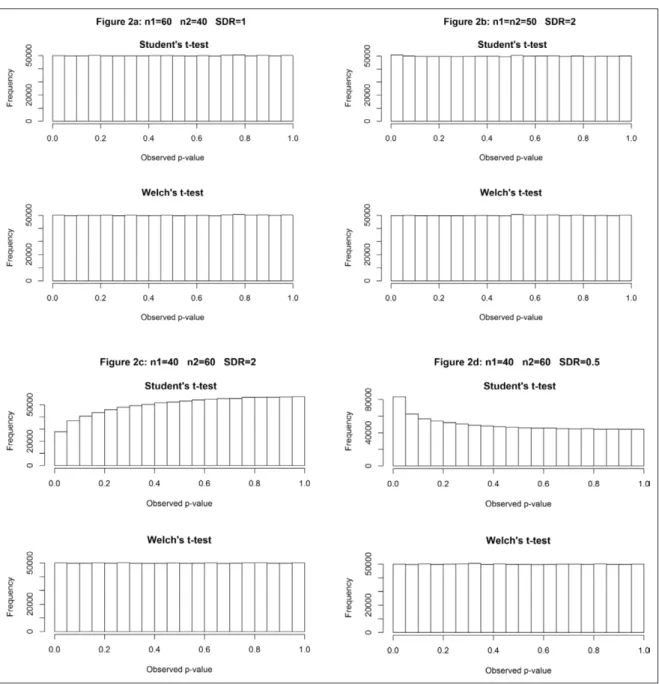
To illustrate the differences in Type 1 error rates between Student’s t-test and Welch’s t-test, we simulated 1,000,000 studies under the null hypothesis (no difference between
Furthermore, we simulated Scenario 3, where both sam-ple sizes and variances were unequal between groups and the larger variance is associated with the larger sample size (SDR = 2; see Figure 2c), and a similar Scenario 4, where
the larger variance is associated with the smaller sample size (SDR = 0.5; see Figure 2d). P-value distributions for
both Student’s and Welch’s t-tests were then plotted. When there is no true effect, p-values are distributed uniformly.
As long as the variances are equal between groups or sample sizes are equal, the distribution of Student’s
p-values is uniform, as expected (see Figures 2a and 2b),
which implies that the probability of rejecting a true null hypothesis equals the alpha level for any value of alpha. On the other hand, when the larger variance is associated with the larger sample size, the frequency of p-values less than 5 percent decreases to 0.028 (see Figure 2c), and
when the larger variance is associated with the smaller sample size, the frequency of p-values less than 5 percent increases to 0.083 (see Figure 2d). Welch’s t-test has a
more stable Type 1 error rate (see Keselman et al., 1998; Keselman, Othman, Wilcox, & Fradette, 2004; Moser & Stevens, 1992; Zimmerman, 2004) Additional simulations, presented in the additional file, show that these scenarios are similar for several shapes of distributions (see tables A3.1 to A3.9 and table A4 in the additional file).
Moreover, as discussed previously, with very small SDRs, Welch’s t-test still has a better control of Type 1 error rates than Student’s t-test, even if neither of them give critical values (i.e., values under 0.025 or above 0.075, according to the definition of Bradley, 1975). With SDR = 1.1, when the larger variance is associated with the larger sample size, the frequency of Student’s p-value being less than 5 percent decreases to 0.046, and when the larger variance is associated with the smaller sample size, the frequency of Student’s p-value being less than 5 percent increases to
0.054. On the other side, the frequency of Welch’s p-values being below 0.05 is exactly 5 percent in both cases.
Yuen’s t-test is not a good unconditional alternative because we observe an unacceptable departure from the nominal alpha risk of 5 percent for several shapes of distributions (see tables A3.1, A3.4, A3.7, A3.8, and A3.9 in the additional file), particularly when we are studying asymmetric distributions of unequal shapes (see tables A3.8 and A3.9 in the additional file). Moreover, even when Yuen’s Type 1 error does not show a critical departure from the nominal alpha risk (i.e., values above 0.075), Welch’s t-test more accurately controls the Type 1 error rate (see tables A3.2, A3.3, A3.5, and A3.6 in the additional file). The Type 1 error rate of Welch’s t-test remains closer to the nominal size (i.e., 5%) in all the previously dis-cussed cases and also performs better with very extreme SDRs and unbalanced designs, as long as there are at least 10 sub-jects per groups (See table A4 in the additional file).
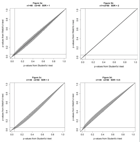
In Figure 3, p-values from Welch’s t-test and Student’s t-test
tests, shown separately in Figure 2 (through histograms), are
now plotted against each other. Figure 3a shows Student’s
p-values plotted against Welch’s p-values of Scenario 1, where
the variance is the same in each group (SDR = 1) and sam-ple sizes are unequal. Figure 3b displays Student’s p-values
plotted against Welch’s p-values of Scenario 2, where the
tests return the same p-value. The top left quadrant contains all p-values less than 0.05 according to a Student’s t-test, but greater than 0.05 according to Welch’s t-test. The bottom right quadrant reports all p-values less than 0.05 accord-ing to Welch’s t-test, but greater than 0.05 accordaccord-ing to Student’s t-test. The larger the standard deviations ratio and the greater the sample sizes ratio, the larger the difference between p-values from Welch’s t-test and Student’s t-test.
Conclusion
When the assumption of equal variances is not met, Stu-dent’s t-test yields unreliable results, while Welch’s t-test controls Type 1 error rates as expected. The widely recom-mended two-step approach, where the assumption of equal variances is tested using Levene’s test and, based on the outcome of this test, a choice of Student’s t-test or Welch’s
t-test is made, should not be used. Because the statistical
power for this test is often low, researchers will inappropri-ately choose Student’s t-test instead of more robust alterna-tives. Furthermore, as we have argued, it is reasonable to assume that variances are unequal in many studies in psy-chology, either because measured variables are used (e.g., age, culture, gender) or because, after random assignment to conditions, variance is increased in the experimental con-dition compared to the control concon-dition due to the experi-mental manipulation. As it is explained in the additional file, Yuen’s t-test is not a better test than Welch’s t-test, since it often suffers high departure from the alpha risk of 5 per-cent. Therefore, we argue that Welch’s t-test should always be used instead of Student’s t-test.
When using Welch’s t-test, a very small loss in statis-tical power can occur, depending on the shape of the distributions. However, the Type 1 error rate is more stable when using Welch’s t-test compared to Student’s t-test, and Welch’s t-test is less dependent on assumptions that cannot be easily tested. Welch’s t-test is available in practically all statistical software packages (and already the default in R and Minitab) and is easy to use and report. We recommend that researchers make clear which test they use by specify-ing the analysis approach in the result section.
Convention is a weak justification for the current prac-tice of using Student’s t-test by default. Psychologists should pay more attention to the assumptions underlying the tests they perform. The default use of Welch’s t-test is a straightforward way to improve statistical practice.
Notes
1 There is a Type 1 error rate inflation in a few cases
where sample sizes are extremely small and SDR is big (e.g., when n1 = n2 = 3 are sampled from uniform dis-tributions and SDR = 2, the Type 1 error rate = 0.083;
2 This is called the Behren-Fisher problem (Hayes & Cai,
2007).
3 In a simulation that explored Type 1 error rates, we
varied the size of the first sample from 10 to 40 in steps of 10 and the sample sizes ratio and the stand-ard deviation ratio from 0.5 to 2 in steps of 0.5, result-ing in 64 simulations designs. Each design was tested 1,000,000 times. Considering these parameter values, we found that the alpha level can be inflated up to 0.11 or deflated down to 0.02 (see the additional file).
4 Other variants have been proposed, such as the percent
trimmed mean (Lim & Loh, 1996).
5 Because sample sizes are equal for each pair of
sam-ples, which sample has the bigger standard deviation is not applicable. In this way, SDR = X will return the same answer in terms of percent power of Levene’s test as SDR = 1/X. For example, SDR = 2 will return the same answer as SDR = ½ = 0.5.
6 For example, many statistical users believe that the
Mann-Whitney non-parametric test can cope with both normality and homosedasticity issues (Ruxton, 2006). This assumption is false, since the Mann-Whitney test remains sensitive to heterosedasticity (Grissom, 2000; Nachar, 2008; Neuhäuser & Ruxton, 2009).
7 Like Bryk and Raudenbush (1988), we note that
une-qual variances between groups does not systematically mean that population variances are different: stand-ard deviation ratios are more or less biased estimates of population variance (see table A2 in the additional file). Differences can be a consequence of bias in meas-urement, such as response styles (Baumgartner & Steenkamp, 2001). However, there is no way to deter-mine what part of the variability is due to error rather than the true population value.
8 Also known as the Satterwaite’s test, the Smith/Welch/
Satterwaite test, the Aspin-Welch test, or the unequal variances t-test.
Competing Interests
The authors have no competing interests to declare.
Additional File
The additional file for this article can be found as follows: • DOI: https://doi.org/10.5334/irsp.82.s1
Author’s Note
References
Baguley, T. (2012). Serious stats: A guide to advanced
statistics for the behavioral sciences. Palgrave
Macmillan. Retrieved from https://books.google.fr/ books?hl=fr&lr=&id=ObUcBQAAQBAJ&oi=fnd&pg-=PP1&dq=baguley+2012&ots=-eiUlHiCYs&sig=YU UKZ7jiGF33wdo3WVO-8l-OUu8.
Banerjee, A., Chitnis, U., Jadhav, S., Bhawalkar, J. & Chaudhury, S. (2009). Hypothesis testing, type I and
type II errors. Industrial Psychiatry Journal, 18(2), 127. DOI: https://doi.org/10.4103/0972-6748.62274
Baumgartner, H. & Steenkamp, J.-B. E. (2001). Response
styles in marketing research: A cross-national investigation. Journal of Marketing Research, 38(2), 143–156. DOI: https://doi.org/10.1509/ jmkr.38.2.143.18840
Bryk, A. S. & Raudenbush, S. W. (1988).
Hetero-geneity of variance in experimental studies: A challenge to conventional interpretations.
Psy-chological Bulletin, 104(3), 396. DOI: https://doi.
org/10.1037/0033-2909.104.3.396
Carroll, R. J. & Schneider, H. (1985). A note on
Levene’s tests for equality of variances. Statistics &
Probability Letters, 3(4), 191–194. DOI: https://doi.
org/10.1016/0167-7152(85)90016-1
Cowdry, R. W., Gardner, D. L., O’Leary, K. M., Leibenluft, E. & Rubinow, D. R. (1991). Mood
variability: A study of four groups. American Journal
of Psychiatry, 148(11), 1505–1511. DOI: https://doi.
org/10.1176/ajp.148.11.1505
Cumming, G. (2013). Understanding the new
statis-tics: Effect sizes, confidence intervals, and meta-analysis. Routledge. Retrieved from https://
books.google.fr/books?hl=fr&lr=&id=1W6la Nc7Xt8C&oi=fnd&pg=PR1&dq=understandi ng+the+new+statistics:+effect+sizes,+confi dence+intervals,+and+meta-analysis&ots=P uJZVHb03Q&sig=lhSjkfzp4o5OXAKhZ_zYzP9nsr8.
Erceg-Hurn, D. M. & Mirosevich, V. M. (2008). Modern
robust statistical methods: An easy way to maxi-mize the accuracy and power of your research.
American Psychologist, 63(7), 591. DOI: https://doi.
org/10.1037/0003-066X.63.7.591
Feingold, A. (1992). Sex differences in variability in
intel-lectual abilities: A new look at an old controversy.
Review of Educational Research, 62(1), 61–84. DOI:
https://doi.org/10.3102/00346543062001061
Glass, G. V., Peckham, P. D. & Sanders, J. R. (1972).
Con-sequences of failure to meet assumptions underlying the fixed effects analyses of variance and covariance.
Review of Educational Research, 42(3), 237–288. DOI:
https://doi.org/10.3102/00346543042003237
Grissom, R. J. (2000). Heterogeneity of variance in
clinical data. Journal of Consulting and
Clini-cal Psychology, 68(1), 155. DOI: https://doi.
org/10.1037/0022-006X.68.1.155
Hanushek, E. A. & W ößmann, L. (2006). Does
educa-tional tracking affect performance and inequality? Differences- in-differences evidence across countries*.
Economic Journal, 116(510), C63–C76. DOI: https://
doi.org/10.1111/j.1468-0297.2006.01076.x
Hayes, A. F. & Cai, L. (2007). Further evaluating the
condi-tional decision rule for comparing two independent means. British Journal of Mathematical and
Statisti-cal Psychology, 60(2), 217–244. DOI: https://doi.
org/10.1348/000711005X62576
Henrich, J., Heine, S. J. & Norenzayan, A. (2010). Most
people are not WEIRD. Nature, 466(7302), 29–29. DOI: https://doi.org/10.1038/466029a
Hoekstra, R., Kiers, H. & Johnson, A. (2012).
Are assumptions of well-known statistical techniques checked, and why (not)? Frontiers in Psychology, 3, 137. DOI: https://doi.org/10.3389/fpsyg.2012.00137
Keppel, G. (1991). Design and analysis: A researcher’s
handbook. Prentice-Hall, Inc. Retrieved from http:// psycnet.apa.org/psycinfo/1991-98751-000.
Keselman, H. J., Huberty, C. J., Lix, L. M., Olejnik, S., Cribbie, R. A., Donahue, B., Levin, J. R., et al. (1998).
Statistical practices of educational researchers: An analysis of their ANOVA, MANOVA, and ANCOVA anal-yses. Review of Educational Research, 68(3), 350–386. DOI: https://doi.org/10.3102/00346543068003350
Keselman, H. J., Othman, A. R., Wilcox, R. R. & Fradette, K.
(2004). The new and improved two-sample t test.
Psychological Science, 15(1), 47–51. DOI: https://
doi.org/10.1111/j.0963-7214.2004.01501008.x
Kester, S. W. (1969). The communication of teacher
expectations and their effects on the achievement and attitudes of secondary school pupils. University of Oklahoma. Retrieved from https://shareok.org/ handle/11244/2570.
Lakens, D., Hilgard, J. & Staaks, J. (2016). On the
repro-ducibility of meta-analyses: Six practical recommen-dations. BMC Psychology, 4(1), 1. DOI: https://doi. org/10.1186/s40359-016-0126-3
Lim, T.-S. & Loh, W.-Y. (1996). A comparison of tests of
equality of variances. Computational Statistics &
Data Analysis, 22(3), 287–301. DOI: https://doi.
org/10.1016/0167-9473(95)00054-2
Luh, W.-M. & Guo, J.-H. (2007). Approximate sample
size formulas for the two-sample trimmed mean test with unequal variances. British Journal of
Math-ematical and Statistical Psychology, 60(1), 137–146.
DOI: https://doi.org/10.1348/000711006X100491
Moser, B. K. & Stevens, G. R. (1992). Homogeneity of
variance in the two-sample means test. American
Statistician, 46(1), 19–21. DOI: https://doi.org/10.1
080/00031305.1992.10475839
Nachar, N. (2008). The Mann-Whitney U: A test for
assess-ing whether two independent samples come from the same distribution. Tutorials in Quantitative
Methods for Psychology, 4(1), 13–20. DOI: https://
doi.org/10.20982/tqmp.04.1.p013
Neuhäuser, M. & Ruxton, G. D. (2009). Distribution-free
that are robust against variance heterogeneity in k × 2 designs with unequal cell frequencies.
Psycho-logical Reports, 76(3), 1011–1017. DOI: https://doi.
org/10.2466/pr0.1995.76.3.1011
Rakotomalala, R. (2008). Comparaison de populations.
Tests Non Paramétriques, Université Lumiere Lyon,
2. Retrieved from http://www.academia.edu/down- load/44989200/Comp_Pop_Tests_Nonparametr-iques.pdf.
Rasch, D., Kubinger, K. D. & Moder, K. (2011). The
two-sample t test: Pre-testing its assumptions does not pay off. Statistical Papers, 52(1), 219–231. DO: https://doi.org/10.1007/s00362-009-0224-x
Ruxton, G. D. (2006). The unequal variance t-test is an
underused alternative to Student’s t-test and the Mann–Whitney U test. Behavioral Ecology, 17(4), 688–690. DOI: https://doi.org/10.1093/beheco/ ark016
Shaw, R. G. & Mitchell-Olds, T. (1993). ANOVA for
unbal-anced data: An overview. Ecology, 74(6), 1638–1645. DOI: https://doi.org/10.2307/1939922
Sheskin, D. J. (2003). Handbook of parametric and
nonparametric statistical procedures (3rd ed.).
Boca Raton, Florida: CRC Press. DOI: https://doi. org/10.1201/9781420036268
Shields, S. (1975). Functionalism, Darwinism, and the
psychology of women. American Psychologist, 30(7), 739. DOI: https://doi.org/10.1037/h0076948
Student. (1908). The probable error of a mean. Biometrika,
1–25. DOI: https://doi.org/10.1093/biomet/6.1.1
Wallenstein, S., Zucker, C. L. & Fleiss, J. L. (1980). Some
statistical methods useful in circulation research.
Circulation Research, 47(1), 1–9. DOI: https://doi.
org/10.1161/01.RES.47.1.1
Wang, H., Smith, K. P., Combs, E., Blake, T., Horsley, R. D. & Muehlbauer, G. J. (2012). Effect
of population size and unbalanced data sets on
robust statistical methods: Basics with illustrations using psychobiological data. Universal Journal of
Psychology, 1(2), 21–31.
Wilcox, R. R. & Keselman, H. J. (2003). Modern robust
data analysis methods: Measures of central tendency.
Psychological Methods, 8(3), 254. DOI: https://doi.
org/10.1037/1082-989X.8.3.254
Yuen, K. K. (1974). The two-sample trimmed t for unequal
population variances. Biometrika, 61(1), 165–170. DOI: https://doi.org/10.1093/biomet/61.1.165
Zimmerman, D. W. (1996). Some properties of
prelimi-nary tests of equality of variances in the two-sample location problem. Journal of General Psychology, 123(3), 217–231. DOI: https://doi.org/10.1080/00 221309.1996.9921274
Zimmerman, D. W. (2000). Statistical significance levels
of nonparametric tests biased by heterogeneous variances of treatment groups. Journal of General
Psychology, 127(4), 354–364. DOI: https://doi.
org/10.1080/00221300009598589
Zimmerman, D. W. (2004). A note on preliminary tests of
equality of variances. British Journal of
Mathemati-cal and StatistiMathemati-cal Psychology, 57(1), 173–181. DOI:
https://doi.org/10.1348/000711004849222
Zumbo, B. D. & Coulombe, D. (1997). Investigation
of the robust rank-order test for non-normal populations with unequal variances: The case of reaction time. Canadian Journal of
Experimen-tal Psychology/Revue Canadienne de Psycholo-gie Expérimentale, 51(2), 139. DOI: https://doi.
org/10.1037/1196-1961.51.2.139
How to cite this article: Delacre, M., Lakens, D. and Leys, C. (2017). Why Psychologists Should by Default Use Welch’s t-test Instead of Student’s t-test. International Review of Social Psychology, 30(1), 92–101, DOI: https://doi.org/10.5334/irsp.82
Published: 05 April 2017
Copyright: © 2017 The Author(s). This is an open-access article distributed under the terms of the Creative Commons Attribution 4.0 International License (CC-BY 4.0), which permits unrestricted use, distribution, and reproduction in any medium, provided the original author and source are credited. See http://creativecommons.org/licenses/by/4.0/.